Lecture 4
One structure: canonical maps and Lagrangian submanifolds
Course map: G1, step 4 of 9. Lecture 2’s bracket and Lecture 3’s symplectic form are one structure: recovers the Hamiltonian vector field, and . Three things the next two lectures need then follow. Canonical transformations are the maps that preserve , and generating functions produce them. Lagrangian submanifolds, on which vanishes, have dimension at most , which is why Lecture 5 asks for commuting integrals and finds Lagrangian tori. And on any cotangent bundle needs no coordinates, which is what the action integral of Lecture 6 is made of.
4.1 The question
Lecture 2 defined the Hamiltonian vector field from the Poisson bracket, and Lecture 3 defined the symplectic form. The Liouville–Arnold theorem of Lecture 5 needs both at once: it is about the flows of functions in involution, and about the shape of the level set they share. So the question is
what single structure do the bracket and the forms describe — and which submanifolds does it single out?
The structure is itself (§4.2). The maps that preserve it are the canonical transformations (§4.3), and the submanifolds it singles out are the Lagrangian ones (§4.4). The worked example is the two-dimensional oscillator, whose level sets are Lagrangian tori (Example 4.15).
4.2 : one structure, two languages
Lecture 2 defined from the bracket, by (Definition 2.4). On a symplectic manifold there is a second route, which uses no bracket at all.
Definition 4.1 (Hamiltonian vector field, from ). On a symplectic manifold , the Hamiltonian vector field of a smooth function is the unique vector field with (4.1) It exists and is unique at each point by (3.10), and it is smooth because and are.
Any symplectic form gives a bracket
Turn (4.2) round and make it a definition: on any symplectic manifold, put (4.3) It is bilinear and antisymmetric, and satisfies Leibniz because . What is left is Jacobi, and this is where closedness enters.
The Jacobi sum turns out to be , a computation done in the reading below. So the bracket (4.3) satisfies the Jacobi identity exactly when : that is what closedness in Definition 3.15 is for. With Jacobi in hand, the second proof of the engine in Lecture 2 runs unchanged, so Theorem 2.5 and Corollary 2.6 hold on every symplectic manifold.
Jacobi is , proved.
The proof is Lecture 2’s computation of the Jacobi identity with non-constant coefficients: the terms in which a derivative lands on a coefficient no longer vanish, and they assemble into exactly .
Proof. Work in any chart , and write and , an antisymmetric matrix, invertible by non-degeneracy. Set , also antisymmetric.
Step 1: the bracket in coordinates. Condition (4.1) reads for each , whose solution is . So This is Lecture 2’s formula (2.3) — except that is now allowed to vary from point to point.
Step 2: what survives in the Jacobi sum. Expand the cyclic sum. The terms carrying a second derivative of one of cancel exactly as in the proof of Proposition 2.2: that argument used only that is antisymmetric at each point, never that it is constant. What is new are the terms in which a derivative lands on . Collecting them, with repeated indices summed,
Step 3: trade for . Differentiate : , so . Substituting into each of the three terms of and relabelling dummy indices so that every term carries the same three factors of ,
Step 4: recognise . By Definition 3.1, the coefficient of in collects exactly the three terms in the bracket, so it is the component . And since , each of the three factors in is minus a component of a Hamiltonian vector field. Three minus signs and the one in front of make a plus: the last step being the determinant formula (2.15) for a -form evaluated on three vectors. That is (4.4).
If the right-hand side vanishes, and Jacobi holds. Conversely, if Jacobi holds for all , take them among the coordinate functions: the fields are the columns of the invertible matrix , so they span every tangent space, and a -form that vanishes on every triple from a basis is zero.
Example 4.5 (A non-degenerate form that is not closed). On take . It is non-degenerate everywhere, and not closed: . Its bracket looks perfectly reasonable — , , the rest zero — and it is not a Poisson bracket:
Lecture 2 proved the engine from the Jacobi identity alone (Theorem 2.5, second proof, a reading). So the engine runs on any closed non-degenerate -form, and on nothing less: that is the sense in which Lecture 2’s bracket and its forms are one structure.
4.3 Canonical transformations and generating functions
Definition 4.6 (Symplectomorphism). A diffeomorphism is a symplectomorphism if .
In canonical coordinates, with written as , the condition is (4.5) where on the left and are regarded as functions of and substituted — pullback is substitution (§3.4). It is a condition you already know under another name, since the matrix of the pulled-back form is , with the Jacobian of .
Proposition 4.7 (Symplectomorphisms are the canonical transformations). satisfies (4.5) if and only if the new coordinates have canonical brackets, and .
Proof (★). By (3.12) the pulled-back form has matrix , so (4.5) says . On the other hand, by the chain rule and , the brackets of the new coordinates form the matrix , and canonical brackets say . The two conditions are equivalent: either one forces , and inverting gives , which with is ; the converse is the same computation backwards.
For one degree of freedom , so a canonical transformation of the plane is exactly an area- and orientation-preserving map. To check the shear , pull back: . The stretch fails, with . For the condition is much stronger than preserving volume (a reading at the end of this lecture).
Proposition 4.8 (Hamiltonian flows are symplectic proved on ; modulo Darboux in general). For every and every point at which the flow of is defined, .
Proof. First on with the standard form. By Proposition 4.2, in the ordering. The Jacobian of at a point therefore obeys the linearised equation , , with and the (symmetric) Hessian of along the trajectory. Then because and . So for all , which is the claim on ; the reduction of a general symplectic manifold to this case is in the reading.
On a general symplectic manifold the trajectory may leave any one chart, but gives and the bracket is a rate of change at a single point, which may be computed in a Darboux chart there (Theorem 4.18): it is the computation above at , where , and it vanishes.
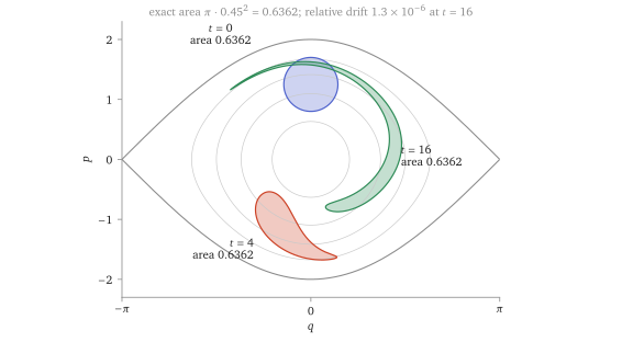
With canonical brackets, Leibniz and the chain rule give and : Hamilton’s equations keep their form.
Generating functions
A transformation given as a formula is easy to check. The problem in practice runs the other way: to produce canonical transformations adapted to a given . Generating functions do this, and the form language says in one line why they work.
Proposition 4.9 (Why generating functions work). Let be a function of old positions and new momenta, and define implicitly by (4.6) wherever are good coordinates. Then (4.5) holds.
Proof. In the coordinates , (4.6) says exactly that Apply . The right-hand side gives (Theorem 3.2); the left gives . So .
That is the mechanism in full: a generating function is a primitive for a combination of canonical -forms, and turns “exact” into “canonical”. For example gives and : shifting every momentum by a gradient is canonical. The function alone gives the identity.
The other classical types work identically. A type-1 function with and says ; for instance gives , which exchanges position and momentum up to a sign. Type 1 cannot generate the identity, whose and are not independent, which is one reason type 2 is the workhorse and the type Lecture 6 uses.
Hamilton–Jacobi, recalled in this language
Hamilton–Jacobi looks for a type-2 generating function adapted to : an with (4.7) for some function of the new momenta alone. The new equations are then and , a constant: conserved momenta, and positions advancing at constant speed. Lecture 6 does this with the actions and the angles. With held fixed, (4.7) also says that the -dimensional set lies inside a level set of — §4.4 returns to this.
4.4 Lagrangian submanifolds
How large can a subspace be on which vanishes?
Let with non-degenerate. The -complement of a subspace is ; by (3.10) it is the preimage of the covectors vanishing on , so (4.8) Unlike an orthogonal complement, can contain , since every vector is -orthogonal to itself. Call isotropic if vanishes on it, i.e. ; then (4.8) gives : an isotropic subspace has dimension at most .
Definition 4.10 (Lagrangian subspace, Lagrangian submanifold). A Lagrangian subspace is an isotropic subspace of the maximal dimension . A submanifold is Lagrangian if it has dimension and for all tangent to — equivalently, if the pullback of to vanishes, written .
This bound is why Lecture 5 asks for exactly integrals.
Proposition 4.11 (At most commuting integrals). If satisfy and are linearly independent at a point, then .
Proof. At that point the vectors are linearly independent, since and is an isomorphism. They span an isotropic subspace, since by (4.2). So .
Seeing it in
In , , the signed areas of the two shadows of the parallelogram on . A plane is Lagrangian when the two shadow areas of a basis parallelogram cancel (Figure 4.2).
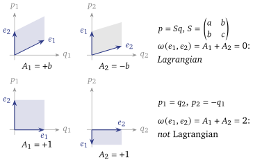
Examples
Example 4.12 (Curves in the plane). For every curve is Lagrangian: it has dimension , and a -form vanishes on parallel vectors. The notion has content from on.
Example 4.13 (Positions and momenta). In the -space and each -space are Lagrangian, since pairs a -direction only with a -direction. The -plane is not: restricts to on it.
The most important examples are graphs, and they bring back Lecture 3.
Proposition 4.14 (Lagrangian graphs are closed -forms). Let be a -form on an open set of -space, and its graph. Then . Hence is Lagrangian if and only if is closed. In particular the graph of , (4.9) is Lagrangian for every function .
Proof. Parametrise by . Pulling back is substituting : by (2.13) and (3.1). For this vanishes by Theorem 3.2.
is called a generating function of the Lagrangian submanifold, and the name is not a coincidence: by (4.7), a solution of Hamilton–Jacobi is a family of Lagrangian graphs, one for each value of , each lying in a level set of . Lecture 6’s is exactly that, with the invariant tori as the family.
By the Poincaré lemma a closed is locally some ; globally it need not be. On the pendulum’s cylinder, with angle , a rotation orbit at energy is the graph of the -form — closed, as every -form on a circle is, and Lagrangian. It is not for any function on the circle, for the reason of Proposition 3.6: . Lecture 6 calls the rotating pendulum’s action. A nonzero action is precisely the obstruction to a global generating function, and Lecture 6 lives in that gap.
Example 4.15 (A Lagrangian torus in ). Take the two-dimensional oscillator’s integrals and, for , the level set a circle in each symplectic plane: a torus (Figure 4.4). Its tangent spaces are spanned by and , each tangent to its own circle and nonzero there, and . So is Lagrangian: each tangent parallelogram has one edge in each symplectic plane, so both its shadows are degenerate.
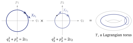
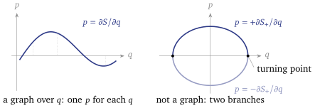
Example 4.15 is Lecture 5’s first proof step, done by hand; the general argument is Proposition 4.11’s, with equality. Like the circle of Figure 4.3, is not a graph over .
4.5 Cotangent bundles and the canonical -form
Positions and their momenta
Let be a configuration space, a manifold of dimension — the circle for the pendulum, the torus for the double pendulum. Its cotangent bundle is the set of pairs a point of configuration space and a covector there. A chart on writes the covector as (Definition 2.7), and is then a chart on the -dimensional . That momenta are covectors shows in a change of chart : writing the same covector in both bases, , forces (4.10) momenta transform like the components of a gradient, not like those of a velocity. For polar coordinates on the plane, (4.10) gives and — the momentum conjugate to the angle is the angular momentum, as it should be.
The canonical -form
Definition 4.16 (Canonical -form). At a point of and for a tangent vector there, (4.11) In words: push down to configuration space, and feed it to the covector — which is part of the point, and so is already there (Figure 4.5).
In a chart, drops the momentum components of , so (4.11) is . The form of Example 2.9, and of Lecture 6’s action integral, is therefore the same -form in every cotangent chart, because (4.11) mentions no chart.
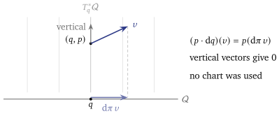
Theorem 4.17 (Every cotangent bundle is symplectic). is a symplectic form on , and in every cotangent chart it is .
Proof. In a chart, , so is the standard form there, which is non-degenerate (Example 3.16). It is closed because it is exact: . And it is the same form in every chart, because is.
So the pendulum’s cylinder, the double pendulum’s and the rigid body’s are symplectic, with no choice made.
The minus sign, and why it costs nothing
The minus sign in comes with the wedge order , which (3.13) showed is the one giving Hamilton’s equations. It is compensated where it matters. Orbits of the oscillator run clockwise in the -plane, a clockwise orbit bounds its disc with the opposite orientation, and the two signs cancel: along the motion is , the enclosed area, which is positive (§3.4 computed it). So the action integral of Lecture 6, taken along the motion, comes out positive.
Point transformations are canonical
A diffeomorphism of configuration space moves momenta by the transpose of its inverse Jacobian — that is (4.10) read as a map — and so lifts to a map of , the cotangent lift. Because is defined without a chart, , and hence by (3.6). Every change of configuration coordinates, with the momenta carried along as covectors, is a canonical transformation. This is why passing to polar coordinates, with the angular momentum, never needs checking. It is also the type-2 generating function of Proposition 4.9, as a one-line computation with (4.6) confirms.
4.6 What it buys
The count in the definition of integrability. At most independent functions Poisson-commute (Proposition 4.11), because their Hamiltonian vector fields span a subspace on which vanishes. So is the most one can ask for, and Lecture 5 asks for exactly that.
The shape of the invariant tori. The oscillator’s level sets are Lagrangian tori (Example 4.15). Lecture 5 proves the same of every compact connected component of a common level set of functions in involution on which their differentials are independent.
The tool for action–angle variables. A type-2 generating function produces a canonical transformation (Proposition 4.9), and a solution of Hamilton–Jacobi is a family of Lagrangian graphs. Lecture 6 builds the action–angle variables from such an .
A chart-free . On any cotangent bundle the canonical -form needs no coordinates (Definition 4.16), and (Theorem 4.17), so the action integral of Lecture 6 is the same in every chart.
4.7 Caveats, in one place
Status. Of the results the lectured core uses, three are proved only in readings: the Jacobi identity for the bracket of , that symplectomorphisms are the maps with canonical brackets (Proposition 4.7), and that Hamiltonian flows are symplectic. So the engine and Corollary 2.6 on a general symplectic manifold rest on two reading proofs, this lecture’s and the second proof of the engine in Lecture 2. Darboux’s theorem is sketched, and its version adapted to commuting functions is cited, both in a reading. Propositions 4.2, 4.9, 4.11 and 4.14 and Theorem 4.17 are proved in the lectured core.
Generating functions are local. Proposition 4.9 holds where are good coordinates. A closed -form need not have a global primitive, and Lecture 6’s changes branch at the turning points (Figure 4.3).
4.8 Darboux’s theorem: no local invariants
Theorem 4.18 (Darboux sketched). Every point of a -dimensional symplectic manifold has a chart around it in which . (da Silva, §8.1; Arnold, §43.)
Such a chart is a Darboux chart, or canonical coordinates. So any statement about alone — or about the bracket and the fields built from it — that is proved in ’s and ’s holds near every point of every symplectic manifold.
What “no local invariants” means — and what it does not
Compare a Riemannian metric, which measures lengths and angles. A sphere of radius has curvature at every point, and curvature is a local invariant: no chart, however small, makes the sphere’s metric into the flat . Darboux’s theorem says a symplectic form has nothing of the kind (Figure 4.6): every small patch of every -dimensional symplectic manifold is indistinguishable from every other, and the dimension is the only local invariant there is.
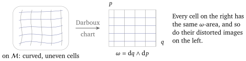
It is easy to hear “no local invariants” as “nothing interesting happens”, and that is the opposite of the point: everything interesting is global. It lives in loops that do not bound, in regions of finite size, in how charts are glued together — never at a point. The actions of Lecture 6 are integrals over loops, and the tori of Lecture 5 are compact; neither is visible in a Darboux chart.
Why it is true: Moser’s idea
At a single point, linear algebra already makes standard (the reading proves this). Call that constant form and join it to by the straight line , . Near the point each is non-degenerate, and is closed, hence by the Poincaré lemma (Theorem 3.4). Now look for a flow that pulls every back to . Its velocity is forced: , which non-degeneracy solves. That this does the job is one differentiation, which uses and a formula for differentiating a form along a flow that we cite (reading). Then carries to , and its coordinates are a Darboux chart.
At a point it is linear algebra; near a point it is Moser
Lemma 4.19 (Linear Darboux). Let be a non-degenerate antisymmetric bilinear form on a vector space . Then has a basis with and . In particular .
Proof. Pick any . By non-degeneracy some has ; rescale it to . On the form is non-degenerate, and its -complement has dimension and meets only in . So , and is still non-degenerate on : a vector there pairing to zero with all of also pairs to zero with , hence with . Repeat inside .
Lemma 4.19 makes standard at one point by a linear change of coordinates. A metric can be pushed a little further — suitable coordinates make it Euclidean at a point to first order — but no further: at second order its curvature is in the way. A symplectic form can be made standard on a whole neighbourhood, and that is Theorem 4.18. The proof spends closedness in exactly one place.
Proof of Theorem 4.18 (sketch: Moser’s trick). Work in a chart around a point in which, by Lemma 4.19, agrees at with the constant form . Join them by , . Each is closed, and equals at , so it is non-degenerate on a small ball around . On that ball is closed, hence exact by the Poincaré lemma (Theorem 3.4): , and can be chosen to vanish at by subtracting its constant part. Define a time-dependent vector field by ; it exists by non-degeneracy and vanishes at , so its flow fixes and is defined near up to . The one tool used without proof is Cartan’s formula for the rate of change of a form along a flow (da Silva, §6.1), which gives Closedness is spent in the middle term. So , and the coordinates composed with are a Darboux chart for .
Theorem 4.20 (Darboux, adapted to commuting functions cited). Let be functions with and linearly independent at a point. Near that point there are functions such that is a Darboux chart: . (Bolsinov–Fomenko, Lemma 1.1, stated there in their convention .)
In such a chart the are momenta and the positions, so by Proposition 4.2 : the commuting flows are translations at unit speed. That is the whole of the Liouville–Arnold theorem locally, and it costs nothing — as Babelon, Bernard and Talon remark (ch. 2, Remark 2), near any point where Darboux gives canonical coordinates with , so every Hamiltonian is “integrable” on a small enough patch.
So Lecture 5 is not trivial. Its question is whether the continue over a whole level set, and what they do when they are continued: they come back to themselves, which makes them angles and the level set a torus. Action-angle coordinates are an adapted Darboux chart on a whole neighbourhood of a torus, and the global part is what Lecture 5 and Lecture 6 add.
4.9 The Liouville volume , and more than volume
Proposition 4.21 (The Liouville volume form). In canonical coordinates, (4.12) which as a measure is the phase-space volume of Liouville’s theorem (an exercise), . In particular is nowhere zero, on any symplectic manifold, since a Darboux chart exists around every point.
Proof. Expanding by bilinearity, a term with a repeated index repeats a -form and vanishes. The survivors are the orderings of the -forms , which commute by (2.16) and so are all equal. Reordering into costs a sign , which a measure does not see.
Theorem 4.22 (Liouville, in one line as Proposition 4.8). For any region and any for which is defined on all of , , where is the measure of .
Proof. By Proposition 4.8 and the rule (3.6), . Now change variables in the integral, being an orientation-preserving diffeomorphism onto its image: .
This is Liouville’s theorem on phase-space volume (an exercise), now a consequence of the stronger . For the two coincide; for the symplectic statement is strictly stronger.
Theorem 4.23 (Poincaré’s integral invariant proved modulo Stokes). Let be a closed loop in and let be defined on it. Then
The proof, Stokes on the tube the loop sweeps out (Figure 4.7), is in the reading.
Proof. Sweep the loop along the flow: maps the cylinder into phase space, with . Orient by ; its induced boundary is then the top loop minus the bottom one, so Stokes (Theorem 3.11) applied on , as in Corollary 3.13, gives using . Relative to the integrand has coefficient , by (4.1). At each fixed this is the derivative of a periodic function of , so its integral over vanishes; by Fubini, so does .
The same holds on any cotangent bundle, since the proof used only two facts that hold there globally: (Theorem 4.17) and (Definition 4.1).
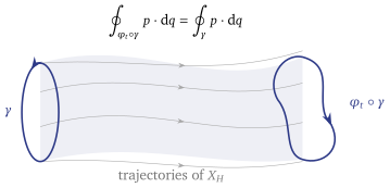
For this is Liouville again; for it conserves the sum of the signed areas of the loop’s shadows, counted with winding number (a figure-eight shadow contributes the difference of its lobes), not a volume. It is the prototype of the action variable: Lecture 6 integrates around a cycle on an invariant torus, and the flow carries the cycle to another with the same integral.
Theorem 4.24 (Gromov non-squeezing cited). A symplectomorphism can map a ball of radius in into the cylinder only if . (Gromov, Invent. Math. 82, 1985.)
For the cylinder has infinite volume, so this is symplectic, not volumetric — and not local, since it concerns a ball of definite size. We shall not use it.
The cross-section must be a -plane. Over the -plane the symplectic map squeezes a ball of radius into , as thin as you like.
Summary
- One structure. recovers Lecture 2’s , with (Proposition 4.2), and the bracket of satisfies Jacobi because .
- Canonical transformations are the maps with , and generating functions produce them because (Proposition 4.9).
- Lagrangian submanifolds: dimension , . At most independent functions commute (Proposition 4.11); graphs of closed -forms and the oscillator’s tori are Lagrangian (Proposition 4.14, Example 4.15).
- Cotangent bundles are symplectic with no choice made, and (Theorem 4.17).
- Next: Lecture 5 proves the Liouville–Arnold theorem. Where integrals in involution are independent, the compact components of their common level sets are tori, and the motion on them is a straight line.
References
da Silva, Lectures on Symplectic Geometry, §§1–4 (symplectic forms, cotangent bundles and the tautological form, Lagrangian submanifolds, generating functions) and §§7–8 (the Moser trick and Darboux); Arnold, Mathematical Methods of Classical Mechanics, §§37–38 and 40–41 (symplectic structures, integral invariants, the Poisson bracket from ), §43 (Darboux), §44 (the integral invariant of Poincaré–Cartan) and §§47–48 (Hamilton–Jacobi, generating functions); Bolsinov and Fomenko, Integrable Hamiltonian Systems, §1.3 (Darboux, and its version adapted to commuting functions). Conventions. da Silva’s agree with ours exactly — with the tautological form, , , and the engine’s minus sign. Arnold and Bolsinov–Fomenko write , so their is minus ours: check any formula from them against (3.13) and Theorem 4.17 before transcribing it.
End of Lecture 4
One structure: canonical maps and Lagrangian submanifolds
Lecture 4 · Contents
Keyboard
- → Space PgDn
- next screen, stopping before an equation, figure or statement it would cut
- ← PgUp
- previous screen
- ↓ ↑ wheel
- scroll freely
- Home End
- the start or the end
- S
- Full ↔ Spine, keeping your place
- T
- Think first on or off
- R
- reveal the next hidden proof
- C
- Core only on or off
- G
- contents: jump to a section or a statement
- + −
- text size
- D
- light or dark
- F
- full screen
- P
- pen on or off: draw on the text
- E
- erase the ink on the screen
- Z double-click
- enlarge an equation, figure or table; Z again for the next
- L
- laser pointer on or off
- B .
- blank the screen
- M
- move the toolbar: right, bottom, left, top
- ?
- this help
- Esc
- close a panel