2.1 The question

Lecture 1 left two jobs. The Liouville–Arnold theorem (Lecture 5) needs $n$ conserved quantities whose flows commute, but Theorem 1.9 speaks of vector fields, not of conserved quantities. And the action variables of Lecture 6 are loop integrals of $p\cdot\dd q$ , which need an integrand that a curve can integrate without a metric. So the question is

in what language is a conserved quantity written, and in what language the loop integral of $p\cdot\dd q$ ?

The answers are the Poisson bracket (§§2.2 and 2.3) and differential forms (§§2.4 and 2.5).

2.2 The Poisson bracket

Definition 2.1 (Poisson bracket). For smooth functions $f,g$ on $T^{*}\R^{n}$ , $\pb{f}{g}\;=\;\sum_{i=1}^{n}\left( \frac{\partial f}{\partial q_i}\frac{\partial g}{\partial p_i} -\frac{\partial f}{\partial p_i}\frac{\partial g}{\partial q_i}\right), \qquad\text{so}\qquad \pb{q_i}{p_j}=\delta_{ij}.$ (2.1)

Proposition 2.2 (The Poisson algebra). The bracket is bilinear, antisymmetric $\pb{f}{g}=-\pb{g}{f}$ , and satisfies the Jacobi identity and the Leibniz rule $\pb{f}{\pb{g}{h}}+\pb{g}{\pb{h}{f}}+\pb{h}{\pb{f}{g}}=0, \qquad \pb{fg}{h}=f\pb{g}{h}+g\pb{f}{h}.$ (2.2)

Proof. Bilinearity and antisymmetry are visible in (2.1), and Leibniz is the product rule applied to each derivative. Jacobi is a line of index bookkeeping, proved in the reading that follows. It uses only that the matrix of brackets of the coordinates is constant and antisymmetric.

The Jacobi identity, proved. Write $z^{1},\dots,z^{2n}$ for all the coordinates at once and $\pb{u}{v}=\sum_{\alpha,\beta}\partial_\alpha u\;J^{\alpha\beta}\;\partial_\beta v, \qquad J^{\alpha\beta}=\pb{z^\alpha}{z^\beta},$ (2.3) so that $J$ is a constant and antisymmetric matrix — that is all of (2.1) the argument uses. Expand the cyclic sum. Every term carries a second derivative of exactly one of $f,g,h$ , so the terms fall into three classes, and it is enough to kill one: the others follow by relabelling $f,g,h$ cyclically. Take the class with a second derivative of $h$ . It comes only from the first two summands, since $\pb{h}{\pb{f}{g}}$ differentiates $h$ just once, and it is $\underbrace{\partial_\alpha f\,J^{\alpha\beta}\,\partial_\gamma g\, J^{\gamma\delta}\,\partial_\beta\partial_\delta h}_{\text{from }\pb{f}{\pb{g}{h}}} \;+\; \underbrace{\partial_\alpha g\,J^{\alpha\beta}\,\partial_\beta\partial_\gamma h\, J^{\gamma\delta}\,\partial_\delta f}_{\text{from }\pb{g}{\pb{h}{f}}} ,$ summed over repeated indices. Relabel the dummy indices of the second term by $\alpha\mapsto\gamma$ , $\beta\mapsto\delta$ , $\gamma\mapsto\beta$ , $\delta\mapsto\alpha$ : it becomes $\partial_\alpha f\,\partial_\gamma g\,\partial_\beta\partial_\delta h\, J^{\gamma\delta}J^{\beta\alpha}$ . The two terms now differ only in carrying $J^{\alpha\beta}$ where the other carries $J^{\beta\alpha}$ , so their sum has the factor $J^{\alpha\beta}+J^{\beta\alpha}$ , which vanishes. The class is zero, and so are the other two.

The bracket is what turns §1.3’s geometry back into calculation. For any observable $f$ , the chain rule along a trajectory together with (1.6) gives $\frac{\dd f}{\dd t} =\sum_i\left(\frac{\partial f}{\partial q_i}\dot q_i +\frac{\partial f}{\partial p_i}\dot p_i\right) =\pb{f}{H}.$ (2.4)

Definition 2.3 (First integral). $f$ is a first integral — a conserved quantity — if $\pb{f}{H}=0$ .

So $H$ generates time evolution. $\dd f/\dd t=\pb{f}{H}$ , with the bracket in that order, is the convention of this course, and every sign that follows comes from it.

Noether, in one line

The condition $\pb{f}{H}=0$ is antisymmetric in its two arguments, so it vanishes for the pair $(f,H)$ exactly when it vanishes for $(H,f)$ . Reading (2.4) both ways:

$f$ is conserved by the flow of $H$ $\iff$ $H$ is invariant under the flow of $f$ .

That is Noether’s theorem, at this level of generality, and it is a one-line consequence of antisymmetry. A conserved quantity is a symmetry; they are not two facts related by a theorem but one fact read in two directions. Angular momentum is conserved because $H$ is rotation-invariant, and — the same sentence — rotations are a symmetry because angular momentum is conserved.

2.3 From functions to vector fields: the engine

Lecture 1 attached a vector field to $H$ . The same construction works for any function.

Definition 2.4 (Hamiltonian vector field). For a smooth function $f$ , the Hamiltonian vector field $\hvf{f}$ is defined by its action on functions, $\hvf{f}\,h\;=\;\pb{h}{f},$ (2.5) which in coordinates reads $\hvf{f}=\sum_i\big(\tfrac{\partial f}{\partial p_i}\partial_{q_i} -\tfrac{\partial f}{\partial q_i}\partial_{p_i}\big)$ .

Taking $f=H$ gives $\hvf{H}h=\pb{h}{H}=\dd h/\dd t$ by (2.4), so $\hvf{H}$ is the field (1.7) of Lecture 1. The map $f\mapsto\hvf{f}$ takes functions, with their Poisson bracket, to vector fields, with their Lie bracket. The question is whether it respects the two brackets.

The worked example: the oscillator’s two halves

Split the oscillator’s Hamiltonian, at unit frequency, as $H=\tfrac12(q^{2}+p^{2})=f+g$ with $f=q^{2}/2$ and $g=p^{2}/2$ . Their fields, the Lie bracket of the fields, and the field of their Poisson bracket can each be computed in a line: $\begin{aligned} \hvf{f}&=-q\,\partial_p, &\qquad \hvf{g}&=p\,\partial_q, &\qquad \comm{\hvf{f}}{\hvf{g}}&=-q\,\partial_q+p\,\partial_p,\\[2pt] \pb{f}{g}&=qp, &\qquad \hvf{qp}&=q\,\partial_q-p\,\partial_p, &\qquad \hvf{\pb{f}{g}}&=-\comm{\hvf{f}}{\hvf{g}}. \end{aligned}$ (2.6) So here the map respects the brackets up to a sign, which §2.7 explains. The sum of the two halves is the oscillator, and $\hvf{H}=\hvf{f}+\hvf{g}=p\,\partial_q-q\,\partial_p$ is the rotation of the phase plane; its orbits other than the equilibrium are circles, the positive-energy level curves of §1.4 at unit frequency. The engine says that what happened here happens for every pair of functions.

Theorem 2.5 (The engine). For all smooth $f,g$ , $\hvf{\pb{f}{g}}\;=\;-\comm{\hvf{f}}{\hvf{g}} .$ (2.7)

The proof is a computation in coordinates. A second proof, three lines long and from the Jacobi identity, shows why it is true; it is a reading.

First proof, in coordinates. Take $n=1$ ; the general case is the same with sums over $i$ . Write subscripts for partial derivatives, so $\hvf{f}=f_p\,\partial_q-f_q\,\partial_p$ . For vector fields $A=a\,\partial_q+b\,\partial_p$ and $B=c\,\partial_q+d\,\partial_p$ , Proposition 1.8 gives $\comm{A}{B}=(Ac-Ba)\,\partial_q+(Ad-Bb)\,\partial_p$ . With $a=f_p,\;b=-f_q,\;c=g_p,\;d=-g_q$ the $\partial_q$ component of $\comm{\hvf{f}}{\hvf{g}}$ is $\hvf{f}g_p-\hvf{g}f_p =\big(f_pg_{qp}-f_qg_{pp}\big)-\big(g_pf_{qp}-g_qf_{pp}\big).$ On the other side, $\pb{f}{g}=f_qg_p-f_pg_q$ , so the $\partial_q$ component of $\hvf{\pb{f}{g}}$ is $\pb{f}{g}_p=f_{qp}g_p+f_qg_{pp}-f_{pp}g_q-f_pg_{qp},$ which is the negative of the previous display, term for term. The $\partial_p$ components are the identical computation and give $\hvf{f}(-g_q)-\hvf{g}(-f_q) =f_{qq}g_p+f_qg_{pq}-f_{pq}g_q-f_pg_{qq} =\pb{f}{g}_q ,$ against $-\pb{f}{g}_q$ for $\hvf{\pb{f}{g}}$ — again a sign apart. Hence $\comm{\hvf{f}}{\hvf{g}}=-\hvf{\pb{f}{g}}$ .

Second proof, from the Jacobi identity. Apply both sides to an arbitrary function $h$ and use only (2.5). The right-hand side is $\comm{\hvf{f}}{\hvf{g}}h =\hvf{f}\pb{h}{g}-\hvf{g}\pb{h}{f} =\pb{\pb{h}{g}}{f}-\pb{\pb{h}{f}}{g}.$ The left-hand side is $\pb{h}{\pb{f}{g}}$ , and the Jacobi identity (2.2), rearranged with antisymmetry, says exactly $\pb{h}{\pb{f}{g}}=\pb{\pb{h}{f}}{g}-\pb{\pb{h}{g}}{f}$ . The two sides are therefore negatives of each other, for every $h$ .

The second proof locates the content: the engine is the Jacobi identity, wearing different clothes. The map $f\mapsto\hvf{f}$ is an anti-homomorphism of Lie algebras, and it is one because the bracket satisfies Jacobi — which is also, as a reading of Lecture 4 shows, the same statement as $\dd\symp=0$ .

Only two properties of $J$ were used, that it is constant and antisymmetric, so the Jacobi identity has nothing to do with the particular pairing of each $q$ with its own $p$ . Lecture 3 meets the same fact in geometric clothes: antisymmetry becomes $\symp$ being a $2$ -form, and constant coefficients make $\dd\symp=0$ automatically. Closedness without constancy is enough, and it is what corresponds to Jacobi in general.

What the course actually uses

Corollary 2.6 (Commuting integrals, commuting flows). If $\pb{F_i}{F_j}=0$ then $\comm{\hvf{F_i}}{\hvf{F_j}}=0$ , and if in addition the fields are complete, their flows commute.

Proof. $\hvf{\pb{F_i}{F_j}}=\hvf{0}=0$ , so Theorem 2.5 gives $\comm{\hvf{F_i}}{\hvf{F_j}}=0$ ; then apply Theorem 1.9.

What the corollary buys is large. It converts an algebraic hypothesis that can be checked — $n$ functions whose brackets vanish — into a geometric conclusion: $n$ commuting vector fields, each tangent to the common level sets of the functions, since $\hvf{F_j}F_i=\pb{F_i}{F_j}=0$ . On a compact regular component of a level set the fields are complete (Proposition 1.7, applied to the component), so their flows commute and together give an action of the abelian group $\R^{n}$ on it. That action is the whole machine of the Liouville–Arnold theorem in Lecture 5, and Theorem 2.5 is what starts it.

2.4 Why forms: $1$ -forms and the cotangent space

The object we are trying to build

In Lecture 6 we shall meet the integral $I \;=\; \frac{1}{2\pi}\oint_{\gamma} p\cdot\dd q \;=\; \frac{1}{2\pi}\oint_{\gamma}\ \sum_{i=1}^{n} p_i\,\dd q_i ,$ (2.8) taken around a closed loop $\gamma$ on an invariant torus, and everything in Lectures 5 and 6 depends on it being a well-defined number. Three separate things have to be true, and not one of them is obvious:

The integrand must be an object that a curve can integrate, with no extra structure supplied. In particular no length, no angle, no inner product: phase space has no metric, and any construction that secretly uses one is not available to us.
The answer must not change when the curve is reparametrised. A loop traversed quickly and the same loop traversed slowly must give the same number.
The answer must not change when $\gamma$ is deformed. Otherwise (2.8) labels a curve rather than a torus, and there is no “action variable” at all.

This lecture settles the first by getting the type of the integrand right: $p\cdot\dd q$ is a $1$ -form. Lecture 3 settles the second, since line integrals of $1$ -forms do not see the parametrisation, and proves what the third needs: the integral of a closed $1$ -form round a loop does not change when the loop is deformed. That $p\cdot\dd q$ is closed on the tori where (2.8) is taken — compact connected components of common level sets of $n$ conserved quantities in involution, on which their differentials are independent — is proved in Lecture 5, and Lecture 6 then defines the actions.

Covectors

Throughout this lecture $\phase$ is a smooth manifold of dimension $m$ , and $x^1,\dots,x^m$ is a chart on it. In the application $\phase$ is phase space and $m=2n$ , with $n$ the number of degrees of freedom — $n$ is reserved for that throughout the course, so it is not available here.

Recall from §1.2 that a tangent vector at $p\in\phase$ is the velocity of a curve through $p$ , equivalently a derivation on functions near $p$ , and that these form an $m$ -dimensional vector space $T_p\phase$ . The chart gives $T_p\phase$ the basis $\partial/\partial x^1,\dots,\partial/\partial x^m$ .

Definition 2.7 (Covector, cotangent space). A covector at $p$ is a linear map $\alpha_p\colon T_p\phase\to\R$ . The set of them is the cotangent space $T_p^{*}\phase$ , the dual of $T_p\phase$ ; it is again a vector space of dimension $m$ . A differential $1$ -form $\alpha$ on $\phase$ assigns to each point $p$ a covector $\alpha_p$ , smoothly in $p$ .

The example to hold on to is the differential of a function.

Definition 2.8 (The differential of a function). For $f$ smooth near $p$ and $v\in T_p\phase$ , set $\dd f_p(v) \;=\; v(f),$ (2.9) the derivative of $f$ along $v$ . This is linear in $v$ , so $\dd f_p\in T_p^{*}\phase$ , and $\dd f$ is a $1$ -form.

Applying (2.9) to the coordinate functions $x^i$ themselves gives $\dd x^i(\partial/\partial x^j)=\partial x^i/\partial x^j=\delta^i_j$ : the $1$ -forms $\dd x^1,\dots,\dd x^m$ are exactly the basis of $T^{*}_p\phase$ dual to the coordinate basis of $T_p\phase$ . Hence every $1$ -form is $\alpha \;=\; \sum_{i} a_i(x)\,\dd x^i , \qquad\text{and in particular}\qquad \dd f \;=\; \sum_i \frac{\partial f}{\partial x^i}\,\dd x^i ,$ (2.10) the second identity being (2.9) evaluated on each basis vector. So the notation $\dd f$ , which until now was a formal symbol in the chain rule, is a genuine object: a machine that eats a tangent vector and returns a number.

The picture: a stack of surfaces

A tangent vector is drawn as an arrow. A covector is not an arrow; it is a stack. Draw the level sets $f=c$ , $f=c+1$ , $f=c+2$ , … near $p$ : for a nearly-constant $f$ they are far apart, for a rapidly varying $f$ they are close together (Figure 2.1). Then (2.9) says

$\dd f_p(v)$ is the number of level surfaces the arrow $v$ pierces.

Figure 2.1. A covector is a stack, not an arrow. The same function drawn where it varies slowly and where it varies fast:

\dd f

is denser where

f

changes quickly. Nothing in the picture requires a notion of length — only the surfaces and their labels.

Figure 2.2.

\dd f_p(v)

counts the level surfaces pierced by

v

. The long arrow

w

gives the smaller answer: it is the crossing of surfaces that is measured, not the length of the arrow.

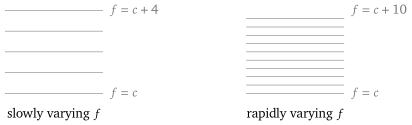
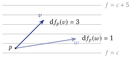
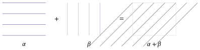
Figure 2.2 shows why no metric is needed. Nothing in the counting used how long $v$ is or what angle it makes with anything; a covector is exactly the structure that can be evaluated on a vector with no metric present. Addition of covectors is superposition of stacks (Figure 2.3): $\alpha+\beta$ is denser than either.

Figure 2.3. Adding covectors superposes stacks. The sum runs in a new direction and is denser than either summand, which is the geometric content of

(\alpha+\beta)(v)=\alpha(v)+\beta(v)

Example 2.9 (The canonical $1$ -form, met early). On $\phase=T^{*}\R^{n}$ with coordinates $q_1,\dots,q_n,p_1,\dots,p_n$ , the expression $\sum_i p_i\,\dd q_i$ is a $1$ -form: at each point of phase space it eats a tangent vector $v$ and returns $\sum_i p_i\,\dd q_i(v)$ , the momenta contracted with the $q$ -components of $v$ . It is emphatically not of the form $\dd f$ — that is the subject of Lecture 3, and the reason (2.8) is ever nonzero. Lecture 4 will show that this $1$ -form exists on any cotangent bundle without choosing coordinates.

2.5 $2$ -forms, oriented area and the wedge product

What we want to measure

A $1$ -form measures a curve’s worth of information: one vector in, one number out. To integrate over a surface we need a machine taking two vectors, and it should return the area of the parallelogram they span — because that is what a surface integral adds up.

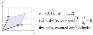
Start in the plane, where the answer is already known from linear algebra: the parallelogram spanned by $v=(v^1,v^2)$ and $w=(w^1,w^2)$ has signed area $A(v,w)\;=\;\det\begin{pmatrix} v^1 & w^1\\ v^2 & w^2\end{pmatrix} \;=\; v^1w^2-v^2w^1 .$ (2.11) Three properties of $A$ are worth naming before we generalise, because they are forced by what “area” means and not chosen for convenience.

Bilinearity. Doubling one edge doubles the area; gluing two parallelograms along an edge adds their areas.
$A(v,v)=0$ . A degenerate parallelogram has no area.
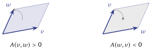
$A(w,v)=-A(v,w)$ . The area is signed: it records not only how much area there is but which way round the two edges run.

The third property is the one students find arbitrary, so note that it is not an extra assumption: it follows from the first two. Expanding $0=A(v+w,v+w)=A(v,v)+A(v,w)+A(w,v)+A(w,w)$ gives $A(v,w)=-A(w,v)$ at once. Antisymmetry is what you get for free once you ask that a degenerate parallelogram have zero area.

Figure 2.4. The same parallelogram, the same area, opposite orientations. A

2

-form remembers the circulation arrow, and that memory is exactly the minus sign in

\alpha\wedge\beta=-\beta\wedge\alpha

Definition 2.10 ( $2$ -form). A $2$ -form at $p$ is a bilinear map $\beta_p\colon T_p\phase\times T_p\phase\to\R$ with $\beta_p(v,w)=-\beta_p(w,v)$ . A differential $2$ -form assigns such a $\beta_p$ to each point, smoothly.

The wedge product

Two $1$ -forms produce a $2$ -form in exactly one natural way.

Definition 2.11 (Wedge product of $1$ -forms). For $1$ -forms $\alpha,\beta$ , $(\alpha\wedge\beta)(v,w)\;=\;\alpha(v)\,\beta(w)-\alpha(w)\,\beta(v) \;=\;\det\begin{pmatrix}\alpha(v) & \alpha(w)\\ \beta(v)&\beta(w)\end{pmatrix}.$ (2.12)

Antisymmetry in $(v,w)$ is manifest, so $\alpha\wedge\beta$ is a $2$ -form; and swapping the two forms transposes the determinant, so $\alpha\wedge\beta=-\beta\wedge\alpha, \qquad\text{and in particular}\qquad \alpha\wedge\alpha=0 .$ (2.13) This is the same minus sign as Figure 2.4, now in the algebra. It is worth saying out loud that (2.13) is a statement about orientation, not a convention about symbols: a plane with a circulation arrow drawn on it is a different object from the same plane with the arrow reversed, and $\wedge$ is the product that knows the difference.

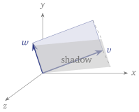
Example 2.12 ( $\dd x\wedge\dd y$ is the signed area). Take $\alpha=\dd x$ , $\beta=\dd y$ in the plane. Then $(\dd x\wedge\dd y)(v,w)=v^1w^2-v^2w^1$ , which is precisely (2.11): see Figure 2.5. The abstract definition has reproduced the determinant, and we may now stop writing $A$ .

Figure 2.5.

\dd x\wedge\dd y

evaluated on two vectors. The number returned is the signed area of the parallelogram they span, in units of the cell

\partial_x,\partial_y

— positive here because

v,w

run anticlockwise.

In $m$ dimensions, a $2$ -form has components $\beta_{ij}=\beta(\partial_i,\partial_j)$ with $\beta_{ij}=-\beta_{ji}$ , so $\beta \;=\; \sum_{i<j}\beta_{ij}\;\dd x^i\wedge \dd x^j ,$ (2.14) a sum over $\binom{m}{2}$ independent components. In the plane there is one, $\dd x\wedge\dd y$ ; in $\R^{3}$ there are three; in $\R^{4}$ , six — and it is the $\R^{4}$ count that Lecture 3 will need when it writes $\symp=\dd q_1\wedge\dd p_1+\dd q_2\wedge\dd p_2$ .

Figure 2.6.

(\dd x\wedge\dd y)(v,w)

is the signed area not of the parallelogram but of its shadow in the

xy

-plane. A

2

-form does not measure area; it measures area as seen in a chosen pair of directions, which is why there is one

2

-form per pair of coordinates.

Higher degree, and the one rule we need

The pattern of (2.12) continues. A $k$ -form is a multilinear map on $k$ tangent vectors that changes sign whenever two arguments are swapped, and the wedge of $k$ $1$ -forms is the determinant of the matrix of pairings: $(\alpha^{1}\wedge\cdots\wedge\alpha^{k})(v_1,\dots,v_k) \;=\;\det\!\big[\alpha^{i}(v_j)\big]_{i,j=1}^{k} .$ (2.15) One more rule is needed, because (2.15) covers only wedges of $1$ -forms: the wedge of forms of any degree, which the exterior derivative of Lecture 3 uses.

Definition 2.13 (Wedge in general). The wedge product is bilinear and associative, and on products of $1$ -forms it simply concatenates the factors, $(\alpha^{1}\wedge\cdots\wedge\alpha^{k})\wedge (\beta^{1}\wedge\cdots\wedge\beta^{\ell}) =\alpha^{1}\wedge\cdots\wedge\alpha^{k}\wedge\beta^{1}\wedge\cdots\wedge\beta^{\ell}.$ Since every form is a sum of such products of coordinate differentials, those two rules determine it. Moving one factor past another costs a sign each time, so in degrees $k$ and $\ell$ $\eta\wedge\xi=(-1)^{k\ell}\,\xi\wedge\eta .$ (2.16) In particular a form of odd degree wedged with itself vanishes, while one of even degree need not.

Example 2.14 ( $\symp^{2}$ , computed). With $\symp=\dd q_1\wedge\dd p_1+\dd q_2\wedge\dd p_2$ on $\R^{4}$ , expanding bilinearly gives four terms. The two like terms vanish, because $\dd q_i\wedge\dd p_i\wedge\dd q_i\wedge\dd p_i$ repeats a factor, and the two cross terms are equal by (2.16) with $k=\ell=2$ . So $\symp\wedge\symp=2\,\dd q_1\wedge\dd p_1\wedge\dd q_2\wedge\dd p_2, \qquad\text{that is}\qquad \frac{\symp^{2}}{2!}=\dd q_1\wedge\dd p_1\wedge\dd q_2\wedge\dd p_2 .$ The factorial in the Liouville volume $\symp^{n}/n!$ , a reading in Lecture 4, is there to cancel exactly this count, and nothing more.

2.6 What it buys

A test for commuting flows that can be computed. Functions whose brackets vanish have commuting fields (Corollary 2.6), and commuting flows when the fields are complete. That is the hypothesis of Lecture 5, in a form that a calculation can settle.
The type of $p\cdot\dd q$ . It is a $1$ -form (Example 2.9), so a curve can integrate it with no metric. Lecture 3 differentiates and integrates forms, and proves that the loop integral of a closed $1$ -form depends on the loop only through its class; Lecture 5 shows that $p\cdot\dd q$ is closed on the tori where it will be integrated. Lecture 3 and Lecture 4 then show that the two halves of this lecture are one structure, the symplectic form, a $2$ -form.

2.7 Caveats, in one place

Status. The Jacobi identity in Proposition 2.2 is proved in a reading; the rest of that proposition, the engine and its corollary are proved in the lectured core, except that the corollary’s last clause, commuting flows, rests on Theorem 1.9, which is cited.
The sign. (2.7) carries a minus sign because of the convention $\dd f/\dd t=\pb{f}{H}$ of (2.4), together with (2.5). Sources that write $\hvf{f}h=\pb{f}{h}$ , or put the bracket of the evolution law the other way round, print a plus, and they make no different claim about mechanics. Corollary 2.6, the consequence that the proof of the Liouville–Arnold theorem uses, does not see the sign.
Coordinates. The bracket (2.1) is defined here on $T^{*}\R^{n}$ , in the coordinates $(q,p)$ . That the same bracket makes sense on any phase space, in any canonical chart, is Lecture 4’s.

Summary

The bracket. $\dd f/\dd t=\pb{f}{H}$ (2.4), and a first integral is $\pb{f}{H}=0$ . By antisymmetry, “ $f$ is conserved by $H$ ” and “ $H$ is invariant under $f$ ” are one statement: Noether in one line.
The engine. $\hvf{\pb{f}{g}}=-\comm{\hvf{f}}{\hvf{g}}$ (Theorem 2.5), checked on the oscillator’s two halves (2.6). Its consequence: commuting integrals give commuting flows (Corollary 2.6).
$1$ -forms eat vectors and need no metric. A covector is a stack of surfaces, $\dd f_p(v)$ counts the surfaces that $v$ pierces, and $p\cdot\dd q$ is a $1$ -form.
$2$ -forms measure oriented area. The wedge (2.12) builds them from $1$ -forms, and $\alpha\wedge\beta=-\beta\wedge\alpha$ records orientation; it is not a convention.
Next: Lecture 3 differentiates and integrates forms, proves Stokes’ theorem, and defines the symplectic form.

Worked in the tutorial: Exercise Sheet 2.

References

Arnold, Mathematical Methods of Classical Mechanics, Ch. 8 (Hamiltonian vector fields, the Lie algebra of Hamiltonian functions) and §32 (exterior algebra); da Silva, Lectures on Symplectic Geometry, §§1–3 and 18 (Poisson structures) and §6 (forms); Babelon, Bernard and Talon, Introduction to Classical Integrable Systems, Ch. 1. Sign conventions differ across all three sources for precisely the identity of §2.3: check any formula against (2.7) and (2.6) before transcribing it.

The whole bibliography, lecture by lecture →

Two languages: the Poisson bracket and differential forms

What this lecture does

2.1 The question