1.1 Why a manifold

The pendulum’s phase space is a cylinder

A plane pendulum is described by an angle $\theta$ and its conjugate momentum $p$ . It is tempting to say the phase space is $\R^{2}$ , and for most purposes nothing goes wrong. But $\theta$ and $\theta+2\pi$ are the same configuration, not two different ones, so the honest phase space is $\phase \;=\; S^{1}\times\R ,$ (1.1) a cylinder: the circle of angles, times the line of momenta.

This is not pedantry, and it is worth seeing the difference immediately. Take the Hamiltonian in units where the length, mass and gravity are $1$ , $H(\theta,p)=\tfrac12 p^{2}-\cos\theta ,$ (1.2) and ask what the level set $H=E$ looks like for $E>1$ — a pendulum swinging right over the top.

On $\R^{2}$ : two curves, $p=\pm\sqrt{2(E+\cos\theta)}$ , each running off to $\theta=\pm\infty$ without ever meeting itself. The angle grows without bound, and the trajectory is not periodic — nor is it a bounded set.
On the cylinder: each of the two becomes a single closed curve, winding once around. The motion is periodic, with a period you can compute (an exercise; Lecture 6 computes the period of the swinging pendulum).

The same disagreement runs the other way below the separatrix: for $-1<E<1$ the plane shows infinitely many congruent ovals, one around each point $(2\pi k,0)$ , where the cylinder shows one oval, which is the one physical orbit.

A theorem that says “the motion is periodic” cannot even be stated on the wrong space. Lecture 5, whose whole content is that the motion runs on a torus, is unstateable without this vocabulary. So the question of this lecture is

where do the states of a mechanical system live, and how do they move — in terms that do not depend on the coordinates?

The answer comes in three steps: the states live on a manifold (this section); motion is a vector field on it, followed along its integral curves (§1.2); and Hamilton’s equations are one such field (§1.3). The pendulum is the worked example throughout, and §1.4 draws its phase portrait.

Charts

The circle is the smallest space that cannot be covered by one coordinate. The angle $\theta$ is a perfectly good coordinate on $S^1$ minus a point, but carry it all the way round and it jumps by $2\pi$ ; and there is no way to choose the cut so that this does not happen somewhere. Two overlapping charts suffice (Figure 1.1), and the price of the second chart is the whole apparatus of a manifold.

Figure 1.1. A chart on

S^{1}

. The circle is the smallest example of a space that needs more than one coordinate patch, and the pendulum lives on it.

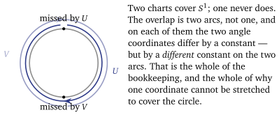
Definition 1.1 (Smooth manifold, in the form we need). A smooth manifold $\phase$ of dimension $m$ is a space covered by charts — one-to-one maps from open pieces of $\phase$ onto open subsets of $\R^{m}$ — such that wherever two charts overlap, the map between their coordinates is smooth with smooth inverse. A function on $\phase$ is smooth if it is smooth in every chart, which is well defined precisely because the transitions are.

Throughout Part I, $\phase$ is the phase space of a mechanical system, and it is a manifold of dimension $m=2n$ , where $n$ is the number of degrees of freedom. That is the only thing $n$ ever means in this course; where a statement is about a general manifold and $2n$ would be misleading, the dimension is called $m$ .

Example 1.2 (Three phase spaces, and what they are not).

Plane pendulum: configuration space $S^{1}$ , phase space $T^{*}S^{1}=S^{1}\times\R$ , dimension $2$ .
Double pendulum: two angles, so configuration space is the torus $T^{2}=S^{1}\times S^{1}$ , and phase space is $T^{*}T^{2}=T^{2}\times\R^{2}$ , dimension $4$ . Emphatically not $\R^{4}$ .
Free rigid body: a configuration is an orientation, so configuration space is the rotation group $SO(3)$ and phase space is $T^{*}SO(3)$ , dimension $6$ . We name it and go no further; $SO(3)$ is not simply connected, and that is a genuine physical fact — but it is not one this course needs.

Each of these is a cotangent bundle, “positions and their momenta”, and Lecture 4 will show that every cotangent bundle carries the structure that makes Hamiltonian mechanics work, for free.

1.2 Tangent vectors, vector fields and flows

Tangent vectors

On a curved space a velocity cannot be an arrow from one point to a distant one; it is the velocity of a curve through the point (Figure 1.2). What can be computed with is what that velocity does to functions.

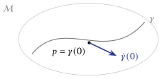
Figure 1.2. A tangent vector is the velocity of a curve through the point. This is the picture to keep; the definition that follows exists because a picture cannot be differentiated.

Definition 1.3 (Tangent vector). A tangent vector at $p$ is a linear map $v$ from smooth functions near $p$ to $\R$ satisfying the Leibniz rule $v(fg)=f(p)\,v(g)+g(p)\,v(f).$ (1.3) Such a map is called a derivation at $p$ . The tangent vectors at $p$ form a vector space $T_p\phase$ of dimension $m$ , and a chart $x^1,\dots,x^m$ gives it the basis $\partial/\partial x^1,\dots,\partial/\partial x^m$ .

A curve $\gamma$ with $\gamma(0)=p$ gives such a derivation, $v(f)\;=\;\frac{\dd}{\dd t}\Big|_{t=0} f(\gamma(t)),$ (1.4) and every derivation arises this way: a tangent vector is the velocity of a curve, acting on functions as a directional derivative.

Why both pictures are needed. The picture of Figure 1.2 is correct and it is the one to hold, but it cannot be computed with: two different curves through $p$ can have the same velocity, and saying which pairs do requires coordinates and an equivalence relation. The computational definition avoids that by recording not the curve but what the curve does to functions. Keep Figure 1.2 as the picture and Definition 1.3 as the tool, and never expect either alone to do both jobs.

Vector fields, integral curves and flows

Definition 1.4 (Vector field, integral curve, flow). A vector field $X$ assigns a tangent vector $X_p\in T_p\phase$ to each point, smoothly; in a chart, $X=\sum_i X^i(x)\,\partial/\partial x^i$ . An integral curve of $X$ is a curve with $\dot\gamma(t)=X_{\gamma(t)}$ . The flow $\varphi_t$ sends a point $p$ to $\gamma(t)$ , where $\gamma$ is the integral curve through $p$ at $t=0$ .

In a chart the integral-curve condition is the system $\dot x^i=X^i(x)$ : an ordinary differential equation, which is why the following is assumed rather than proved.

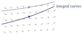
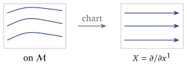
Theorem 1.5 (Existence and uniqueness cited). Through each point of $\phase$ there is exactly one integral curve of a smooth vector field $X$ , defined for at least a short time, and it depends smoothly on its starting point. Where both sides are defined, the flow satisfies $\varphi_{t+s}=\varphi_t\circ\varphi_s$ and $\varphi_0=\id$ .

Figure 1.3. A vector field, and two of its integral curves. The arrows are given; the curves are what you get by following them. Theorem 1.5 says exactly one curve passes through each point.

Near a point where $X\ne0$ the flow can be straightened: there are coordinates in which $X=\partial/\partial x^1$ and the integral curves are parallel straight lines (Figure 1.4). Nothing local distinguishes one non-vanishing vector field from another — all the content is global, a theme that returns as Darboux’s theorem, in a reading of Lecture 4.

Figure 1.4. The flow box. Wherever

X\ne0

there is a chart in which the flow is translation at unit speed: a non-vanishing vector field has no local invariants at all.

Completeness

Theorem 1.5 promises an integral curve only for a short time. It may not last: on $\R$ , $\dot x=x^{2}$ has, for $x_0>0$ , the solution $x(t)=x_0/(1-x_0t)$ , which escapes to infinity as $t\to1/x_0$ , although nothing is wrong with the vector field.

Definition 1.6 (Complete). $X$ is complete if every integral curve is defined for all $t\in\R$ — equivalently, if $\varphi_t$ is defined on all of $\phase$ for every $t$ .

Proposition 1.7 (Compactness rescues completeness sketched). A smooth vector field on a compact manifold is complete.

Proof (sketch). Suppose an integral curve exists on a maximal interval $[0,T)$ with $T$ finite. The standard escape argument says such a curve must eventually leave every compact subset — otherwise Theorem 1.5, applied at a limit point, extends it past $T$ and contradicts maximality. On a compact $\phase$ there is nothing to leave. Hence $T=\infty$ .

The Lie bracket

Two vector fields can be composed as differential operators, but $XY$ is not a vector field: applied to a product it produces second derivatives and fails (1.3). The antisymmetric combination survives.

Proposition 1.8 (The Lie bracket). For vector fields $X,Y$ , the operator $\comm{X}{Y}f\;=\;X(Yf)-Y(Xf)$ (1.5) is again a vector field, with components $\comm{X}{Y}^i=X(Y^i)-Y(X^i)$ in any chart.

Proof. Linearity is clear. For Leibniz, expand both terms on a product: $X\big(Y(fg)\big)=X\big(f\,Yg+g\,Yf\big) = f\,X(Yg)+g\,X(Yf)+(Xf)(Yg)+(Xg)(Yf),$ and the same with $X$ and $Y$ exchanged. The two cross terms $(Xf)(Yg)+(Xg)(Yf)$ are symmetric under that exchange, so they cancel in the difference, leaving $\comm{X}{Y}(fg)=f\,\comm{X}{Y}g+g\,\comm{X}{Y}f$ . Those cross terms — note that they are products of first derivatives — are the obstruction to the Leibniz rule, and antisymmetry is exactly what removes them. The genuine second-derivative terms disappear separately and for a different reason: in coordinates they are $(X^iY^j-Y^iX^j)\,\partial_i\partial_j f$ , whose coefficient is antisymmetric in $i,j$ while the Hessian is symmetric. The component formula follows by taking $f=x^i$ .

What the bracket measures is the failure of the two flows to commute: follow $X$ for time $t$ , then $Y$ for time $s$ , then back along each, and the point you return to differs from where you started at order $ts$ , by $\comm{X}{Y}$ . We need only the extreme case, and we need it as an input to Lecture 5.

Theorem 1.9 (Commuting fields, commuting flows cited). Two complete vector fields have commuting flows, $\varphi^X_t\circ\varphi^Y_s=\varphi^Y_s\circ\varphi^X_t$ for all $s,t$ , if and only if $\comm{X}{Y}=0$ . (Arnold, Ch. 8.)

1.3 Hamilton’s equations as one vector field

Now specialise to $\phase=T^{*}\R^{n}$ with coordinates $q_1,\dots,q_n,p_1,\dots,p_n$ , and let $H$ be a Hamiltonian. Hamilton’s equations $\dot q_i=\frac{\partial H}{\partial p_i}, \qquad \dot p_i=-\frac{\partial H}{\partial q_i}$ (1.6) are $2n$ scalar equations, and they are exactly the statement that the trajectory is an integral curve of the single vector field $\hvf{H}\;=\;\sum_{i=1}^{n}\left( \frac{\partial H}{\partial p_i}\frac{\partial}{\partial q_i} -\frac{\partial H}{\partial q_i}\frac{\partial}{\partial p_i}\right).$ (1.7) That is the whole of §1.3: a mechanical system is a manifold with a vector field on it, and solving it means following the arrows.

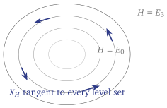
One consequence is immediate and is worth drawing. Apply (1.7) to $H$ itself: the two terms cancel in pairs, so $\hvf{H}H=0$ . Energy is conserved, and geometrically:

$\hvf{H}$ is everywhere tangent to the level sets of $H$ .

A trajectory can never leave the level set it starts on (Figure 1.5). That much is unconditional. How much more it buys depends on the level, and the distinction is worth stating now, because Lecture 5 builds a hypothesis out of it.

At a point where $\dd H\ne0$ — equivalently, by (1.7), where $\hvf{H}\ne0$ — the level set is locally a smooth surface of dimension $2n-1$ . At a critical point of $H$ it need not be a surface at all.

One degree of freedom, on a level where $\dd H\ne0$ : each connected component is a curve, and since $\hvf{H}$ is a nowhere-zero field tangent to it, that component is a single orbit. This is the entire solution of the problem — but note both hypotheses. A level set with several components is several orbits, and a level through a critical point is not covered at all.
$n\ge2$ : a single conserved quantity confines the motion to a $(2n-1)$ -dimensional surface, again only where $\dd H\ne0$ , and no further. That is why Lecture 5 asks for $n$ integrals rather than one — and why it asks for the level set to be regular.

The qualification is not hypothetical: the pendulum’s level $E=1$ in §1.4 crosses itself at a critical point, and it is the lecture’s principal worked example.

Figure 1.5. Level sets of

H

, with

\hvf{H}

tangent to them. Because

\hvf{H}H=0

, a trajectory is trapped on the level set it starts on. For the harmonic oscillator these curves are the orbits, and the picture is the complete solution.

1.4 Worked phase portraits

For one degree of freedom §1.3 has already solved every problem qualitatively: away from the critical points of $H$ , the orbits are the connected components of its level curves, traversed in the direction of $\hvf{H}$ . Two portraits are worth having by heart — and the second is interesting precisely where that qualification bites.

The harmonic oscillator, $H=\tfrac12(p^{2}+\freq^{2}q^{2})$ . For $E>0$ the level sets are ellipses about the origin, all closed, all traversed clockwise; the period is $2\pi/\freq$ and does not depend on which ellipse. That independence is special, and Lecture 6 will see it break. The level $E=0$ is the origin alone — the one critical point, an equilibrium and not an ellipse.

The pendulum, $H=\tfrac12p^{2}-\cos\theta$ on the cylinder (1.1), is the richer picture (Figure 1.6) and the course’s standing example. Three regimes, separated by one curve:

$-1<E<1$ : libration. Closed curves encircling $(\theta,p)=(0,0)$ ; the bob swings back and forth.
$E=1$ : the separatrix. Here $p^{2}=2(1+\cos\theta)=4\cos^{2}(\theta/2)$ , so $p=\pm2\cos(\theta/2)$ for $\theta\in(-\pi,\pi)$ — the range the cylinder coordinate runs over, and the range on which $\cos(\theta/2)\ge0$ makes the square root come out without a modulus. This level is the one place where the warning of §1.3 bites: $\theta=\pi$ , $p=0$ is a critical point of $H$ , so the level set is not a curve there — two branches cross — and it is not one orbit. It is three: the equilibrium itself, and the two curves that leave it and return to it, each taking infinitely long at both ends. Nothing on this level is periodic, though it is drawn as a closed curve on the page.
$E>1$ : rotation. Curves winding around the cylinder, $p$ never changing sign; the bob goes over the top for ever.

Figure 1.6. The pendulum’s phase cylinder. The left and right edges are the same line: a rotation curve leaving on the right returns on the left, and is a single closed orbit. The separatrix (heavy) divides libration from rotation and belongs to neither. The three dots are equilibria — stable at

\theta=0

, unstable at

\theta=\pm\pi

, which on the cylinder is one point, not two. The two regimes are genuinely different curves: period and action calculations use a different cycle in each, and are evaluated separately.

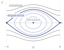
The separatrix is where the two families of closed curves fail to be deformable into one another, and it is the first sign of something this course returns to repeatedly: the interesting structure of an integrable system sits at the places where its level sets change character. Lecture 6 computes the period of libration, and watches the period diverge as the separatrix is approached from either side.

1.5 What it buys

Three things, each used later.

One degree of freedom is solved. Away from the critical points of $H$ , the orbits are the connected components of the level curves (§1.3), and §1.4 drew them for the oscillator and the pendulum. Lecture 6 finds, for the closed ones, the variables in which the motion is uniform.
With $n\ge2$ degrees of freedom, one conserved quantity is not enough. It confines the motion to a level set of dimension $2n-1$ and no further. Lecture 5 asks for $n$ of them, and Lecture 2 supplies the language in which “ $n$ conserved quantities that do not disturb one another” can be written.
Two tools for that theorem. Flows on a compact level set run for all time (Proposition 1.7), and flows whose vector fields have vanishing Lie bracket commute (Theorem 1.9). Together they let $n$ such flows act on a level set as a single action of $\R^{n}$ , which is where the proof in Lecture 5 starts.

1.6 Caveats, in one place

Status. Existence and uniqueness (Theorem 1.5) and commuting flows (Theorem 1.9) are cited, and completeness on a compact manifold (Proposition 1.7) is sketched. The Lie bracket (Proposition 1.8) and $\hvf{H}H=0$ are proved. Some further standard facts are used without proof, among them the tangent-space facts in Definition 1.3 (the dimension, the basis, and that every derivation comes from a curve), the regular-level facts of §1.3 (a regular level set is a smooth surface, by the implicit function theorem; for one degree of freedom a connected piece of a regular level curve is a single orbit), the meaning of the Lie bracket as the order- $ts$ failure of two flows to commute, the infinite time taken along the separatrix, and the oscillator’s period.
Completeness is a hypothesis. Without compactness a smooth vector field need not be complete, as $\dot x=x^{2}$ shows. Lecture 5 asks for compact level sets for exactly this reason. Where they are not compact, as for the Toda ring of Lecture 9, completeness has to be proved by hand.
One field on the cylinder. (1.7) is written in the coordinates $(q,p)$ of $T^{*}\R^{n}$ , and the pendulum uses it in an angle chart $(\theta,p)$ . $H$ is a function on the cylinder because it is $2\pi$ -periodic in $\theta$ . On each connected piece of the overlap of two angle charts, the charts differ by a constant shift of $\theta$ , with $p$ unchanged, and Hamilton’s equations keep their form under such a shift. So (1.7) gives the same vector field in either chart: $\hvf{H}$ is one vector field on the whole cylinder.

Summary

Phase space is a manifold. The pendulum’s is the cylinder $S^{1}\times\R$ , not $\R^{2}$ (1.1), and on the cylinder a rotating pendulum has one periodic orbit rather than infinitely many curves.
Dynamics is a vector field. Hamilton’s equations are the single field $\hvf{H}$ of (1.7). Since $\hvf{H}H=0$ , trajectories are trapped on level sets of $H$ , and for one degree of freedom the regular level curves are the orbits (Figure 1.6).
Completeness. Integral curves can run out of time; on a compact manifold they cannot (Proposition 1.7).
Commuting flows. Two complete flows commute if and only if the Lie bracket of their fields vanishes (Theorem 1.9).
Next: Lecture 2 writes conserved quantities in two languages, the Poisson bracket and differential forms, and turns “the Lie bracket of the flows vanishes” into a statement about the conserved quantities themselves.

Worked in the tutorial: Exercise Sheet 1.

References

Arnold, Mathematical Methods of Classical Mechanics, Ch. 8 (vector fields and their flows on a manifold); da Silva, Lectures on Symplectic Geometry, §§1–3 (manifolds and vector fields); Babelon, Bernard and Talon, Introduction to Classical Integrable Systems, Ch. 1.

The whole bibliography, lecture by lecture →

Phase space and flows

What this lecture does