7.1 The question

Lecture 6 made the motion of an integrable system free in action–angle variables, on tori labelled by the actions. Real systems are at best close to integrable. So the question is

what happens to the tori when an integrable system is perturbed — and how do you see it?

Two theorems answer the first half, one destructive and one constructive; the section map answers the second. The worked example is Hénon–Heiles (§7.6), set beside the Toda ring that Lecture 8 and Lecture 9 will solve.

7.2 Poincaré’s non-existence theorem

Imported from Lecture 6: near a torus of an integrable system there are action–angle coordinates $(\varphi,I)$ , $\varphi\in T^{n}$ , $I$ in an open set $D\subset\R^{n}$ , in which $H=H_0(I)$ and the motion is $\dot\varphi=\freq(I)=\partial H_0/\partial I$ , $\dot I=0$ (Theorem 6.5, Corollary 6.4). $H_0$ is non-degenerate if $\det(\partial^{2}H_0/\partial I^{2})\ne0$ , and then, for $n\ge2$ , the resonant tori of Definition 6.9 are dense and of measure zero (Figure 6.7).

Poincaré called the following the fundamental problem of dynamics: a nearly integrable system $H(\varphi,I)=H_0(I)+\varepsilon H_1(\varphi,I)+O(\varepsilon^{2}), \qquad H_1=\sum_{k\in\Z^{n}}h_k(I)\,e^{\ii k\cdot\varphi},$ (7.1) with $\varepsilon$ small and $H_1$ expanded in a Fourier series in the angles. The planets are the original case: $H_0$ is the motion of each planet round the Sun, and $\varepsilon H_1$ their mutual attraction.

Example 7.1 (Two rotors in a weak periodic potential). On $T^{2}\times\R^{2}$ , with the positions $q\in T^{2}$ themselves the angles and $p=I$ , let $H=\tfrac12\abs{p}^{2}+\varepsilon V(q), \qquad H_0=\tfrac12\abs{I}^{2},\qquad \freq(I)=I .$ Here $\partial^{2}H_0/\partial I^{2}$ is the identity: non-degenerate. Two choices of $V$ will do different things.

$V=\cos q_1+\cos q_2$ separates: $F=\tfrac12p_1^{2}+\varepsilon\cos q_1$ is an exact second integral, and the system is integrable for every $\varepsilon$ .
$V=P_r(q_1)P_r(q_2)$ , where $P_r(x)=(1-r^{2})/(1-2r\cos x+r^{2})=\sum_{m\in\Z}r^{\abs m}e^{\ii mx}$ for a fixed $0<r<1$ . Then $h_k=r^{\abs{k_1}+\abs{k_2}}$ : every Fourier coefficient is nonzero.¹

What separates the two cases is which Fourier modes act on which resonant tori.

Definition 7.2 (Poincaré set, $n=2$ ). The Poincaré set $\mathfrak P\subset D$ of (7.1) is the set of $I$ at which some $k\in\Z^{2}\setminus\{0\}$ has $k\cdot\freq(I)=0\qquad\text{and}\qquad h_k(I)\ne0 :$ the resonant tori on which a Fourier mode of the perturbation resonates.

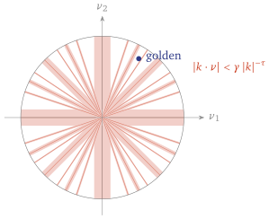
For general $n$ , $I\in\mathfrak P$ asks for $n-1$ linearly independent such $k$ . In Example 7.1, $k\cdot\freq(I)=k\cdot I=0$ is a line through the origin of the $I$ -plane. With $V=\cos q_1+\cos q_2$ only $k=\pm(1,0),\pm(0,1)$ have $h_k\ne0$ , and $\mathfrak P$ is the two axes. With $V=P_rP_r$ every rational line through $0$ is in $\mathfrak P$ : it is dense.

Theorem 7.3 (Poincaré; in Kozlov’s form cited). Let $H(\varphi,I,\varepsilon)$ be real-analytic on $T^{n}\times D\times(-\varepsilon_0,\varepsilon_0)$ , with $H(\varphi,I,0)=H_0(I)$ non-degenerate on $D$ , and let the Poincaré set $\mathfrak P$ be dense in $D$ . Then Hamilton’s equations have no first integral $F=F_0(\varphi,I)+\varepsilon F_1(\varphi,I)+\varepsilon^{2}F_2(\varphi,I)+\cdots,$ a formal power series in $\varepsilon$ with smooth coefficients, that is independent of $H$ .

Here independent is Definition 5.1 read order by order in $\varepsilon$ (Kozlov, ch. IV §1). So the second choice of $V$ in Example 7.1 has no second integral of this kind, and “non-integrable” is a theorem about it, not a report that nobody has found one.

The engine of the proof is visible at first order, and we prove that part in the next section.

7.3 Small denominators

The obvious strategy is to remove $\varepsilon H_1$ by a canonical transformation close to the identity, as Hamilton–Jacobi removed all of $H$ in Lecture 6. Take a type-2 generating function (Proposition 4.9) with old positions $\varphi$ and new momenta $I'$ , $S(\varphi,I')=I'\cdot\varphi+\varepsilon S_1(\varphi,I'), \qquad I=\frac{\partial S}{\partial\varphi}=I'+\varepsilon\frac{\partial S_1}{\partial\varphi}, \qquad \varphi'=\frac{\partial S}{\partial I'}=\varphi+\varepsilon\frac{\partial S_1}{\partial I'} .$ Substitute into (7.1) and expand $H_0(I'+\varepsilon\,\partial_\varphi S_1)$ : $H=H_0(I')+\varepsilon\Big(\freq(I')\cdot\frac{\partial S_1}{\partial\varphi} +H_1(\varphi,I')\Big)+O(\varepsilon^{2}).$ (7.2) The new Hamiltonian is integrable to first order if the bracket does not depend on the angles. Its angle average is $h_0$ , since $\partial_\varphi S_1$ averages to zero; so we need the homological equation $\freq(I')\cdot\frac{\partial S_1}{\partial\varphi}=h_0(I')-H_1(\varphi,I').$ (7.3)

Proposition 7.4 (First-order perturbation theory). On an open set of $I'$ on which $k\cdot\freq(I')\ne0$ for every $k$ with $h_k\ne0$ , and on which the series below converges together with its first and second derivatives, and for $\varepsilon$ small enough, $S_1(\varphi,I')=\sum_{k\ne0}\frac{\ii\,h_k(I')}{k\cdot\freq(I')}\,e^{\ii k\cdot\varphi}$ (7.4) (terms with $h_k=0$ omitted) solves (7.3), and the new Hamiltonian is $H_0(I')+\varepsilon h_0(I')+O(\varepsilon^{2})$ .

Proof. $\freq\cdot\partial_\varphi e^{\ii k\cdot\varphi}=\ii(k\cdot\freq)e^{\ii k\cdot\varphi}$ , so the $k$ -th mode of the left side of (7.3) is $\ii(k\cdot\freq)s_k$ and that of the right side is $-h_k$ . Solve: $s_k=\ii h_k/(k\cdot\freq)$ .²

If $H_0$ is non-degenerate and $H_1$ has finitely many Fourier modes, such open sets exist: everything off the finitely many active resonance hypersurfaces $k\cdot\freq(I')=0$ . If the Poincaré set is dense, as for the second rotor of Example 7.1, no open set qualifies.

Every term is divided by $k\cdot\freq(I')$ , the combination whose vanishing is resonance. On a resonant torus with $h_k\ne0$ — a point of the Poincaré set — the $k$ -th mode of (7.3) reads $0=-h_k$ , and there is no solution at all. Near one the coefficient is enormous. And for $n\ge2$ the resonant tori are dense, so every torus has resonant ones arbitrarily close: these are the small denominators (Figure 7.1). They are not a defect of the method. Near resonance, a small perturbation is not a small change.

Figure 7.1. Small denominators for the rotors of Example 7.1,

V=P_rP_r

r=\tfrac12

: the largest term

\abs{h_k}/\abs{k\cdot\freq}

of (7.4),

\abs{k_1}+\abs{k_2}\le40

, against the frequency ratio. The low-order rationals show as spikes; the truncated sum has a pole at every rational

a/b

with

a+b\le40

, of width shrinking like

r^{a+b}

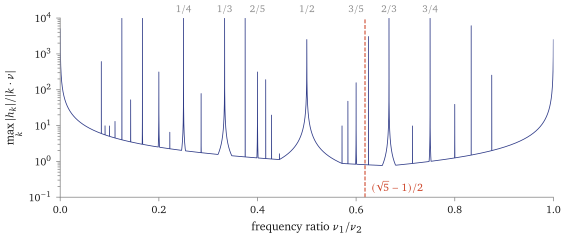
. Most of the line stays low (scripts/figures/small_denominators.py).

The same obstruction kills integrals, which is Poincaré’s point.

Proposition 7.5 (Poincaré’s mechanism at first order). Let $n=2$ , let $H_0$ be non-degenerate, and let $F=F_0+\varepsilon F_1+O(\varepsilon^{2})$ be a first integral of (7.1), with $F_0,F_1$ smooth on $T^{2}\times D$ . Then

$F_0$ depends on $I$ alone;
at every point of $\mathfrak P$ , $\nabla F_0$ is parallel to $\freq$ , that is, $\dd F_0\wedge\dd H_0=0$ .

If $\mathfrak P$ is dense, $\dd F_0\wedge\dd H_0=0$ everywhere: the leading term of every such integral is a function of the energy.

Proof. Expand $\pb{F}{H}=0$ in $\varepsilon$ , with the angles as positions and the actions as momenta.

Order $1$ : $\pb{F_0}{H_0}=\freq\cdot\partial_\varphi F_0=0$ . Its $k$ -th Fourier mode is $\ii(k\cdot\freq)f_{0,k}(I)=0$ , so $f_{0,k}(I)=0$ wherever $\freq(I)$ is non-resonant. Those $I$ are dense, because $H_0$ is non-degenerate (Figure 6.7), and $f_{0,k}$ is continuous, so $f_{0,k}\equiv0$ for $k\ne0$ : $F_0=F_0(I)$ .

Order $\varepsilon$ : $\pb{F_1}{H_0}+\pb{F_0}{H_1}=0$ . The first term is $\freq\cdot\partial_\varphi F_1$ ; the second is $-\nabla F_0\cdot\partial_\varphi H_1$ , since $F_0$ has no angles. The $k$ -th mode:³ $\ii\,(k\cdot\freq)\,f_{1,k}=\ii\,(k\cdot\nabla F_0)\,h_k .$ At $I\in\mathfrak P$ pick the $k$ of Definition 7.2: the left side vanishes and $h_k\ne0$ , so $k\cdot\nabla F_0=0$ . Then $\freq$ and $\nabla F_0$ are both orthogonal to the nonzero vector $k$ of $\R^{2}$ , hence parallel. The last sentence follows by continuity.

7.4 The KAM theorem

Poincaré’s theorem destroys the integrals, but not necessarily the tori. A torus is an invariant set, and it may survive even where no integral does; Proposition 7.4 cannot build it, because of the resonances. The tori to hope for are those furthest from every resonance.

Definition 7.6 (Diophantine). With $\abs k=\abs{k_1}+\dots+\abs{k_n}$ , a frequency vector $\freq\in\R^{n}$ is $(\gamma,\tau)$ -Diophantine if $\abs{k\cdot\freq}\ \ge\ \frac{\gamma}{\abs k^{\tau}} \qquad\text{for every }k\in\Z^{n}\setminus\{0\}.$

It is quantitative non-resonance: every term of (7.4) is then at most $\abs{h_k}\abs k^{\tau}/\gamma$ , which an analytic $H_1$ , with $h_k$ decaying exponentially, easily beats. And almost every vector is Diophantine.

Lemma 7.7 (Diophantine vectors have almost full measure, $n=2$ ). Let $\tau>1$ . In the disc $\abs{\freq}\le R$ of $\R^{2}$ , the vectors that are not $(\gamma,\tau)$ -Diophantine have total area at most $16\sqrt2\,R\,\gamma\,\zeta(\tau)$ , where $\zeta(\tau)=\sum_{m\ge1}m^{-\tau}$ .

Proof (★). For one $k\ne0$ , the bad set $\abs{k\cdot\freq}<\gamma\abs k^{-\tau}$ is a strip about the line $k\cdot\freq=0$ of width $2\gamma\abs k^{-\tau}/\norm k\le2\sqrt2\,\gamma\abs k^{-\tau-1}$ , since the Euclidean length $\norm k\ge\abs k/\sqrt2$ . Inside the disc it has length at most $2R$ , so area at most $4\sqrt2\,R\gamma\abs k^{-\tau-1}$ . There are $4m$ vectors $k$ with $\abs k=m$ . Summing, $\sum_{m\ge1}4m\cdot4\sqrt2\,R\gamma\,m^{-\tau-1}=16\sqrt2\,R\gamma\,\zeta(\tau)$ , which is finite because $\tau>1$ .

Theorem 7.8 (Kolmogorov–Arnold–Moser cited). Let $H=H_0(I)+\varepsilon H_1(\varphi,I)$ on $T^{n}\times D$ , with $H_0$ analytic and $H_1$ analytic and $2\pi$ -periodic in the angles. Let $D_0$ be a bounded region whose closure lies in $D$ , with $H_0$ non-degenerate on a neighbourhood of that closure, and let both functions extend analytically to a complex neighbourhood of fixed width of $T^{n}\times\overline{D_0}$ , where $H_1$ is bounded. Then for sufficiently small $\varepsilon$ , most non-resonant invariant tori of $H_0$ over $D_0$ do not vanish but are only slightly deformed: the perturbed system has invariant tori, densely filled by quasi-periodic orbits with $n$ independent frequencies. They form a majority in the sense that the measure of the part of $T^{n}\times D_0$ they do not cover is small when $\varepsilon$ is small. The theorem guarantees the survival of a large family whose frequencies satisfy a fixed Diophantine condition (Definition 7.6).

7.5 The section map

To see what becomes of the tori we need one tool: the section map.

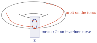
Take $n=2$ and fix the energy, $H=E$ , a three-dimensional level set. Choose a surface $\Sigma$ in it that the flow crosses transversally — for instance $q_1=0$ with $\dot q_1>0$ — with coordinates $(q_2,p_2)$ , the remaining momentum $p_1$ being fixed by $H=E$ . If the orbit from $x\in\Sigma$ comes back to $\Sigma$ , call the first return $P(x)$ : the Poincaré map (Figure 7.2).

Proposition 7.9 (The section map preserves area proved modulo Stokes). For every loop $\gamma$ in $\Sigma$ on which $P$ is defined, the area enclosed in the $(q_2,p_2)$ -plane is the same for $\gamma$ and $P\circ\gamma$ .

The proof is Stokes on the tube of orbits joining $\gamma$ to $P\circ\gamma$ , on which $\symp$ vanishes; it is in the reading.

Proof (★). With $\tau(u)$ the return time of $\gamma(u)$ , the map $(s,u)\mapsto\Phi_{s\tau(u)}(\gamma(u))$ , $s\in[0,1]$ , sweeps a tube $C$ of orbits from $\gamma$ to $P\circ\gamma$ . Both of its tangent vectors are tangent to the level set $H=E$ , and one of them is $\tau\hvf{H}$ . Since $\iota_{\hvf H}\symp=\dd H$ (Definition 4.1), $\symp(\hvf H,v)=\dd H(v)=0$ for every $v$ tangent to the level set, so $\symp$ vanishes on $C$ . By Stokes on $C$ (Theorem 3.11) and $\dd(p\cdot\dd q)=-\symp$ (Theorem 4.17), $\oint_{P\circ\gamma}p\cdot\dd q=\oint_\gamma p\cdot\dd q$ . On $\Sigma$ , $\dd q_1=0$ , so $p\cdot\dd q=p_2\,\dd q_2$ there, and $\oint p_2\,\dd q_2$ is the signed enclosed area. So $P$ preserves area, and orientation with it.

Two readings follow. An invariant torus meets $\Sigma$ in a closed curve, and $P$ maps the curve to itself. And for the unperturbed system, with $\Sigma=\{\varphi_2=0\}$ , coordinates $(\varphi_1,I_1)$ and $\freq_2>0$ (reverse $\varphi_2$ if necessary), the return time is $2\pi/\freq_2$ , in which $\varphi_1$ advances by $2\pi\freq_1/\freq_2$ : $P_0(\varphi_1,I_1)=\big(\varphi_1+2\pi\rho(I_1),\,I_1\big), \qquad \rho=\freq_1/\freq_2\ \text{on the level }H_0=E .$ (7.5) Each circle $I_1=c$ is turned rigidly by $2\pi\rho$ . If $\rho$ changes with $I_1$ — which is what isoenergetic non-degeneracy says — $P_0$ is a twist map: circles at different heights turn by different angles.

Figure 7.2. A Poincaré section: the orbit (red) winds round an invariant torus, and its crossings of

\Sigma

(dots) lie on the curve in which the torus meets

\Sigma

7.6 Poincaré sections: Hénon–Heiles

Hénon and Heiles wanted to know whether a star in an axisymmetric galaxy has a third integral besides the energy and the angular momentum. The question reduces to two degrees of freedom, and they took as the simplest model $H=\tfrac12\big(p_x^{2}+p_y^{2}\big)+\tfrac12\big(x^{2}+y^{2}\big)+x^{2}y-\tfrac13y^{3}.$ (7.6) The potential has a minimum at $0$ and three saddles, at $(0,1)$ and $(\pm\sqrt3/2,-\tfrac12)$ , all at height $1/6$ ; below $E=1/6$ the motion near the origin is confined to a curved triangle.⁴

Its potential is the isotropic oscillator plus a cubic term. Rescaled to a fixed energy, the cubic term’s strength is proportional to $\sqrt E$ (a reading has the computation): the higher the energy, the stronger its effect.

Take the section $\Sigma=\{x=0,\ p_x>0\}$ at fixed $E$ , with coordinates $(y,p_y)$ , and plot the crossings of a dozen orbits (the tutorial at the end of this section has the code). By Proposition 7.9 the picture is a portrait of an area-preserving map, and three kinds of orbit look different:

an orbit on an invariant torus fills a smooth closed curve;
an orbit in an island chain fills several small curves, visited in turn;
a chaotic orbit fills a region, erratically, and its points scatter.

An island chain is what a resonant circle of a perturbed twist map generically breaks into. Every point of a circle with rotation number $a/b$ is fixed by $P^{\,b}$ before the perturbation. After it, the Poincaré–Birkhoff theorem (a reading) guarantees at least two periodic orbits, and in the generic picture there are $2kb$ periodic points for some $k\ge1$ , alternately elliptic, ringed by small closed curves, and hyperbolic, saddles of $P^{\,b}$ . The two curves of points that approach a hyperbolic point, forwards and backwards in time, join into a separatrix in an integrable system; after a perturbation they generically cross, into a homoclinic tangle, which forces chaotic dynamics nearby; the reading computes one for a model twist map, the standard map. The Hénon–Heiles sections below show island chains and scatter that resemble this picture, but they are not a consequence of the theorem: the unperturbed Hénon–Heiles map has a constant rotation number and is no twist map.

Figure 7.3. Sections

x=0

p_x>0

of Hénon–Heiles (7.6) at

E=1/12

1/8

and

1/6

, fourteen orbits each: curves and island chains, then a chaotic sea that at

E=1/6

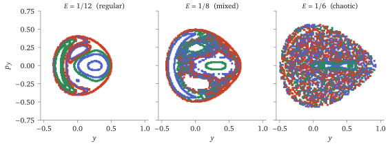
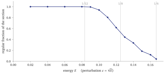
fills most of the section (scripts/figures/henon_heiles_sections.py).

Figure 7.3 is the result, and it is what Hénon and Heiles saw in 1964. At low energy the plotted orbits lie on apparent curves, as if each had a second integral. At higher energies the scatter spreads, and at $E=1/6$ most plotted orbits scatter. A finite-time test classifies launch points as regular or not (Figure 7.4): the fraction classified regular is $1$ to the resolution at small $E$ and falls near $E\approx0.1$ .

Figure 7.4. The regular fraction of the Hénon–Heiles section against the energy: a uniform grid of launch points, each classified by a finite-time Lyapunov exponent (regular if below

0.02

after

t=800

) (scripts/figures/surviving_tori.py).

The code

Take $\Sigma=\{x=0,\ p_x>0\}$ at fixed $E$ , with coordinates $(y,p_y)$ ; the allowed region is $\tfrac12p_y^{2}+\tfrac12y^{2}-\tfrac13y^{3}\le E$ . Launch an orbit from a point of it, with $p_x=\sqrt{2E-p_y^{2}-y^{2}+\tfrac23y^{3}}$ ; integrate Hamilton’s equations accurately; record $(y,p_y)$ each time $x$ passes through $0$ upwards; plot; repeat for a dozen starting points.

The whole computation is a dozen lines of Python.

def rhs(t, z):                      # Hamilton's equations for (eq:6:HH)
    x, y, px, py = z
    return [px, py, -(x + 2*x*y), -(y + x*x - y*y)]
def crossing(t, z): return z[0]     # the section x = 0 ...
crossing.direction = 1              # ... crossed upwards, px > 0

def section(E, y, py, tmax=2000):
    px = sqrt(2*E - py**2 - y**2 + 2*y**3/3)
    s = solve_ivp(rhs, (0, tmax), [0, y, px, py], events=crossing,
                  rtol=1e-10, atol=1e-12)
    return s.y_events[0][:, 1], s.y_events[0][:, 3]   # (y, py)

Two things decide whether the picture can be trusted. The accuracy: $H$ must stay constant along the orbit, and checking it is part of the computation — the generator measures a drift below $10^{-8}$ over $t\approx2000$ , and refuses to draw above $5\times10^{-8}$ . And the event detection: the crossing must be located by root finding on $x(t)=0$ , not by the nearest time step. scripts/figures/henon_heiles_sections.py is this code with a loop over launch points.

7.7 Toda against Hénon–Heiles at equal energy

Three particles on a ring, each pushed by its neighbours through the exponential potential of Toda, with the centre of mass removed and the coordinates, time and energy rescaled (Toda, §2.9), have the Hamiltonian $H_{\mathrm{Toda}}=\tfrac12\big(p_x^{2}+p_y^{2}\big) +\tfrac1{24}\Big(e^{2y+2\sqrt3x}+e^{2y-2\sqrt3x}+e^{-4y}\Big)-\tfrac18 .$ (7.7) This is the periodic Toda chain, a model that Lecture 9 will prove integrable; here we claim nothing else about it. Expand the exponentials: the constants cancel the $-\tfrac18$ , the linear terms cancel ( $2y+2y-4y=0$ ), the quadratic ones give $\tfrac12(x^{2}+y^{2})$ , and the cubic ones give $\tfrac1{144}\Big[(2y+2\sqrt3x)^{3}+(2y-2\sqrt3x)^{3}-64y^{3}\Big] =x^{2}y-\tfrac13y^{3}.$ So $H_{\mathrm{Toda}}$ agrees with Hénon–Heiles (7.6) through cubic order, and differs from it at quartic order.⁵ Hénon–Heiles is the cubic truncation of the Toda chain.

Figure 7.5. The same section

x=0

p_x>0

, at the same energy

E=1/6

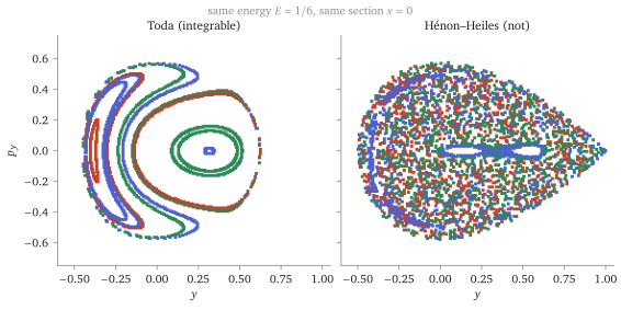
, for the Toda chain (7.7) (left) and its cubic truncation Hénon–Heiles (right). Every plotted Toda orbit lies on a smooth curve; the truncation is mostly chaotic (scripts/figures/toda_vs_henon_heiles.py).

Figure 7.5 puts the two side by side at $E=1/6$ , the highest energy of Figure 7.3. Two Hamiltonians that agree through cubic order disagree about everything that matters. Integrability belongs to the whole Hamiltonian: the cubic Taylor polynomial cannot see it, and it need not survive truncation.

7.8 Lyapunov exponents

Definition 7.10 (Lyapunov exponent). For an orbit $\Phi_t(x_0)$ and a tangent vector $u$ at $x_0$ , $\lambda(x_0,u)=\lim_{t\to\infty}\frac1t\ln\frac{\abs{\dd\Phi_t(u)}}{\abs u},$ where it exists (Ott, §4.4). A positive exponent means exponential sensitivity to the initial condition.

On a torus of an integrable system, in action–angle coordinates $\varphi(t)=\varphi(0)+\freq(I)t$ , so a small change $\delta I$ gives $\delta\varphi(t)=\delta\varphi(0)+t\,(\partial\freq/\partial I)\,\delta I$ : nearby orbits separate linearly, by shear, and every $\lambda$ is $0$ . In a chaotic region they separate exponentially (Figure 7.6). Numerically one computes a finite-time exponent, as in Figure 7.4.

Figure 7.6. Two pairs of Hénon–Heiles orbits at

E=1/8

, each started

10^{-9}

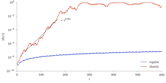
apart: inside an island (blue) they separate linearly, in the chaotic sea (red) exponentially (scripts/figures/lyapunov_separation.py).

7.9 What it buys

Integrability is exceptional, in a stated sense. Poincaré’s theorem rules out a second integral that is a power series in $\varepsilon$ , for a non-degenerate $H_0$ and a dense Poincaré set; and truncating the Toda ring at cubic order turns its regular section at $E=1/6$ into a mostly chaotic one (Figure 7.5). So the integrable systems of Lecture 8 and Lecture 9 have to be found exactly as they are.
The tori are robust. KAM keeps most of them, so an integrable system organises the systems near it.
A diagnostic: a section’s curves against its scatter, and Lyapunov exponents.

7.10 Caveats, in one place

Status. Poincaré’s theorem, KAM and the Poincaré–Birkhoff theorem (a reading) are cited. What is proved is the first-order step of Poincaré’s argument (Proposition 7.5): the leading term of any such integral is a function of $H_0$ , which is not yet non-existence. Proposition 7.4 is proved; Lemma 7.7 is proved in a reading, and Proposition 7.9 in a reading modulo Stokes.
What KAM does not say. No size for “sufficiently small”, no rate for “small”, and no integral. The Diophantine family it guarantees does not fill the resonance zones, and the theorem does not say what is there. The two theorems do not conflict: Poincaré’s rules out an integral of a specified form, and KAM supplies many invariant tori, not an integral.
Hénon–Heiles is outside both theorems. It perturbs the isotropic oscillator, which is degenerate, so neither Theorem 7.3 nor Theorem 7.8, as stated, applies to it. Its sections, and the regular fraction of Figure 7.4, are measurements, not predictions.
A positive Lyapunov exponent alone is not chaos: a hyperbolic periodic point has one. For a bounded orbit that is not periodic it is a numerical indicator, and the threshold in Figure 7.4 is a classifier.
Genericity, and no more. The course puts no measure on the space of all Hamiltonians. It claims Poincaré’s theorem, the effect of truncation in Figure 7.5, and, in a reading, that the integrable members of the Hénon–Heiles family are isolated, for meromorphic integrals.

7.11 Poincaré–Birkhoff, the standard map and the homoclinic tangle

On a circle with $\rho=a/b$ rational (in lowest terms), every point is a fixed point of $P_0^{\,b}$ : the torus is resonant, filled with periodic orbits (Proposition 6.10). On an irrational circle every orbit is dense. Perturb: $P_\varepsilon$ is still area-preserving (Proposition 7.9) and close to $P_0$ . By Theorem 7.8 most of the irrational circles survive as invariant curves. A circle of fixed points is not robust — nothing forces a whole circle of solutions of $P^{\,b}x=x$ to persist — and what remains of it is fixed by a theorem of Poincaré.

Theorem 7.11 (Poincaré’s geometric theorem cited). An area-preserving homeomorphism of a closed annulus to itself that turns its two boundary circles in opposite directions has at least two fixed points.

(Arnold, App. 9: Poincaré announced it just before his death, and Birkhoff proved it.) Apply it between two surviving invariant curves whose rotation numbers $\rho_-<a/b<\rho_+$ straddle the resonance, to $P_\varepsilon^{\,b}$ followed by a rotation by $-2\pi a$ : the inner boundary turns back, the outer forward. The result is periodic orbits of period $b$ that survive the break-up — for a sufficiently small perturbation of an isoenergetically non-degenerate system, at least two geometrically distinct ones (Arnold, App. 9, p. 422).

Two steps hide in “the inner boundary turns back”. Arnold’s hypothesis is pointwise: every point of the inner circle must move backwards. That holds because a circle homeomorphism with rotation number $\rho_-<a/b$ moves every point by less than $2\pi a$ in $b$ steps (if some point moved by exactly $2\pi a$ the rotation number would be $a/b$ ). And the two fixed points of the theorem might lie on one orbit; that there are two distinct periodic orbits coming from this resonant torus is Arnold’s corollary (p. 422): when an $n$ -dimensional torus filled with closed trajectories of an isoenergetically non-degenerate system breaks up under a sufficiently small perturbation, at least $2^{n-1}$ closed trajectories form, counted with multiplicity, of which at least $n$ are geometrically distinct.

In the generic case there are $kb$ periodic points of each of two kinds, and they alternate round the old circle (Ott, §7.2.2): elliptic points, surrounded by small invariant curves of their own, and hyperbolic points, saddles of $P_\varepsilon^{\,b}$ . The resonant torus has become an island chain (Figure 7.7).

Figure 7.7. Poincaré–Birkhoff. Left: in the frame turning with the resonant circle (

\rho=a/b

, dotted), the inner circle

C_-

turns backwards and the outer

C_+

forwards under

P_0^{\,b}

; the dotted circle is fixed pointwise. Right: after the perturbation

C_\pm

survive (KAM) and, of the circle, only the fixed points guaranteed by Theorem 7.11 remain — in the generic case alternately elliptic, ringed by islands, and hyperbolic. Schematic; Figure 7.8 is the computed version.

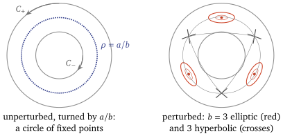
A model twist map, and a homoclinic tangle

The simplest area-preserving perturbation of a twist map is the standard map on the cylinder, $p'=p+K\sin x,\qquad x'=x+p'\qquad(x\bmod2\pi),$ (7.8) the section map of a rotor kicked once per unit time by the potential $K\cos x$ . Its Jacobian has determinant $1$ , and at $K=0$ it is (7.5) with rotation $p$ .⁶ Figure 7.8 shows the whole story: at $K=0.5$ the golden circle survives, deformed, while the resonant circle $\rho=1/3$ has broken into three islands and three hyperbolic points, exactly as Figure 7.7 predicts.

Figure 7.8. The standard map (7.8). Left,

K=0.5

, a band of

p

: most circles survive, deformed (grey); the invariant curve of golden rotation number

(3-\sqrt5)/2

(indigo) is a KAM curve; the resonant circle

\rho=1/3

is gone, replaced by three islands round an elliptic orbit of period

3

(red) and a hyperbolic orbit of period

3

(crosses). Right,

K=0.95

: a chaotic sea, and the golden curve still there. Greene’s numerical evidence suggests that the golden rotational circle is among the last to break, near

K\approx0.9716

(Ott, §7.3.2).

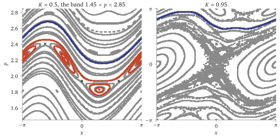
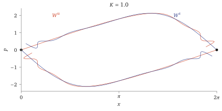
The hyperbolic points carry the chaos. A hyperbolic fixed point has a stable curve $W^{s}$ of points that approach it, and an unstable curve $W^{u}$ of points that approach it backwards in time. In an integrable system they join smoothly into a separatrix, as for the pendulum (§6.4). Perturbed, they generically cross. One crossing $x$ forces infinitely many, since every image $P^{m}x$ is again on both curves; the lobes between successive crossings have equal areas because the map preserves area, and as they crowd towards the fixed point they must stretch into long thin tongues. This homoclinic tangle (Figure 7.9), discovered by Poincaré, forces chaotic dynamics nearby (Ott, §§4.3, 7.2.2): a mechanism for the chaotic dynamics that Figure 7.8 shows, not a computation of that sea’s origin.

Figure 7.9. A homoclinic tangle, computed: the unstable (red) and stable (indigo) curves of the hyperbolic fixed point of the standard map at

K=1

, which sits at both ends (

x=0

and

x=2\pi

are the same point). They do not join into one separatrix; they cross, and the lobes pile up near the fixed point (scripts/figures/homoclinic_tangle.py).

Two consequences of KAM and of the Diophantine condition. For $n=2$ it has a sharp consequence. On a three-dimensional energy level a two-dimensional torus separates, like a surface of revolution in space: an orbit starting between two surviving tori stays between them forever, and its actions stay near their initial values (Arnold, App. 8, p. 407, under the analogous isoenergetic non-degeneracy condition). For $n\ge3$ the tori separate nothing, and a slow drift through the gaps is possible — Arnold diffusion, which we only name.

Figure 7.10. Lemma 7.7. Each resonance

k\cdot\freq=0

(a line through

0

) is thickened to a strip of width

\propto\gamma\abs k^{-\tau-1}

; representative strips with

\abs k\le5

are drawn, not to scale. Every line through

0

with rational slope gets a strip, so the strips are dense, but their total area is

O(\gamma)

: the Diophantine vectors, which lie outside all of them, are almost all.

Positive exponents without chaos. A positive exponent alone is not chaos: the hyperbolic fixed point of the standard map has one. For a bounded orbit that is not periodic, $\lambda>0$ is the standard numerical indicator of chaos, and that is how it is used here.

The energy as the perturbation parameter. The energy is the perturbation parameter. Rescaling $(x,y,p)\mapsto s\,(x,y,p)$ gives $\frac{1}{s^{2}}H(sx,sy,sp) =\tfrac12\big(p_x^{2}+p_y^{2}+x^{2}+y^{2}\big)+s\big(x^{2}y-\tfrac13y^{3}\big),$ so the dynamics at energy $E$ is that of the isotropic oscillator plus a cubic perturbation of size $\varepsilon=s=\sqrt E$ at energy $1$ .

The Hénon–Heiles family. In the family $V_\lambda=\tfrac12(x^{2}+y^{2})+x^{2}y+\tfrac\lambda3y^{3}$ , $\lambda\ne0$ (Hénon–Heiles is $\lambda=-1$ ), the known integrable members are $\lambda=1$ , which separates in the coordinates $(y\pm x)/\sqrt2$ , and $\lambda=6$ , which has a second integral that is a polynomial of degree four, quadratic in the momenta.⁷ For every other $\lambda$ there is no second integral that is meromorphic in the complexified coordinates and momenta — in particular no rational or polynomial one (cited: Ito 1985, completed by Morales-Ruiz, Ramis and Simó 2007). Integrals that are only smooth, or defined on part of phase space, are not excluded. So the statement is: within this family, and for integrals of this class, the integrable members are isolated points of the parameter line.

Summary

The problem: $H=H_0(I)+\varepsilon H_1(\varphi,I)$ (7.1). Poincaré’s theorem (cited): for $H_0$ non-degenerate and a dense Poincaré set there is no second integral that is a power series in $\varepsilon$ .
Small denominators: first-order perturbation theory divides by $k\cdot\freq$ (Proposition 7.4), which vanishes on the dense set of resonances; the same resonances force the leading term of any integral to depend on $H_0$ alone (Proposition 7.5).
KAM (cited): most tori survive, deformed, with Diophantine frequencies, which are almost all (Lemma 7.7).
Sections: the section map preserves area (Proposition 7.9). Curves, island chains and a chaotic sea appear in Hénon–Heiles as the energy grows, while the Toda ring it truncates stays regular at the same energy (Figure 7.5). Lyapunov exponents vanish on tori.
Next: Lecture 8 asks where the Toda ring’s integrals come from, and finds them in a Lax pair.

Worked in the tutorial: Exercise Sheet 7.

References

Arnold, Mathematical Methods of Classical Mechanics, App. 8–9; Kozlov, Russian Math. Surveys 38:1 (1983), ch. IV §1; Ott, Chaos in Dynamical Systems, §§4.4, 7.2–7.3; Toda, Theory of Nonlinear Lattices, §§1.2, 2.9; Hénon and Heiles, Astron. J. 69 (1964) 73; Ito (1985) and Morales-Ruiz, Ramis and Simó (2007) for the Hénon–Heiles family.

The whole bibliography, lecture by lecture →

scripts/check-l6-algebra.py, check 3: the closed form of $P_r$ symbolically, the coefficients sampled.↩︎
scripts/check-l6-algebra.py, check 1, symbolically, including the sign through the type-2 convention of Proposition 4.9.↩︎
scripts/check-l6-algebra.py, check 2, with the frozen bracket.↩︎
scripts/check-l6-algebra.py, check 5.↩︎
scripts/check-l6-algebra.py, check 6, which also checks the reduction from three particles.↩︎
scripts/check-l6-algebra.py, check 8. This is Chirikov’s form; Ott (7.15) kicks after the turn, a conjugate map.↩︎
scripts/check-l6-algebra.py, check 5, which prints it.↩︎

When integrability fails

What this lecture does