6.1 The question

Lecture 5 found angle coordinates on one torus, from its period lattice, and a frequency vector (5.9). It said nothing about how the tori fit together, and its angles are paired with nothing. So the question is

which coordinates make an integrable motion free, and what are its frequencies?

The answer is the action–angle variables of Theorem 6.5. The actions are the loop integrals of $p\cdot\dd q$ over the basis cycles, the angles are conjugate to them, and the frequencies are $\partial K/\partial I$ (Corollary 6.4). The worked example is the librating pendulum (Proposition 6.7), whose frequency, unlike the oscillator’s, depends on its action.

6.2 Action variables, and why they are well defined

We work near one such torus $\Sigma$ , at the value $f$ . The phase space is $\R^{2n}$ or a cotangent bundle, as Proposition 5.12 requires; all three examples below are. One fact about the neighbourhood is imported.

Standing assumption (cited: Arnold, §50 A, the problem there). For $f'$ near $f$ , the component of $\phase_{f'}$ near $\Sigma$ is again a torus satisfying the hypotheses of Theorem 5.7, and the base point $x_0$ and the lattice basis $e_i$ can be chosen to depend smoothly on $f'$ . The smooth lattice basis is the implicit function theorem applied to $\Phi_t(x_0)=x_0$ ; that the nearby components are tori is the content of Arnold’s problem. We write out neither.

Definition 6.1 (Action variables). The action variables of the torus at $f$ are $I_i(f)=\frac{1}{2\pi}\oint_{\gamma_i}p\cdot\dd q,\qquad i=1,\dots,n,$ (6.1) each cycle traversed in the direction of increasing $s$ .

This is the integral (2.8) that Lecture 2 promised. Lecture 2 and Lecture 3 settled the first two of the three things it needs, and the next proposition supplies the third.

Proposition 6.2 (The actions are well defined proved modulo Stokes).

$I_i$ does not change if $\gamma_i$ is replaced by any loop into which it can be deformed within $\Sigma$ . In particular it does not depend on the base point $x_0$ .
$I_i$ depends only on $f$ : it is a function of $F_1,\dots,F_n$ , and so a first integral. The $I_i$ are in involution.

Proof. (1) is Proposition 5.12 together with Corollary 3.13, which rests on Stokes. For the base point: if $x_1=\Phi_\tau(x_0)$ , the loops $s\mapsto\Phi_{u\tau}\big(\Phi_{se_i}(x_0)\big)$ , $u\in[0,1]$ , deform the cycle based at $x_0$ into the cycle based at $x_1$ , inside $\Sigma$ . (2) The definition uses only the torus at $f$ , so $I_i=I_i(F)$ . For two functions of $F$ , Leibniz and the chain rule give $\pb{I_i}{I_j}=\sum_{a,b}\frac{\partial I_i}{\partial f_a} \frac{\partial I_j}{\partial f_b}\pb{F_a}{F_b}=0$ .

A different basis of $\Lambda$ gives different cycles and different actions: the new basis is $e'_i=\sum_jU_{ij}e_j$ with $U$ an integer matrix of determinant $\pm1$ , and $I'=UI$ . There is no preferred choice in general. What never changes is what the actions are for: they are functions of $F$ whose derivatives are the periods.

Proposition 6.3 (The period formula). With $A$ the matrix whose columns are the basis vectors $e_i(f)$ , $2\pi\,\frac{\partial I_i}{\partial f_j}=(e_i)_j, \qquad\text{that is,}\qquad \frac{\partial I}{\partial f}=\frac{1}{2\pi}A^{\mathsf T}.$ (6.2)

Proof. Fix $i$ and $j$ , and sweep the cycle as $f$ moves in direction $j$ : $x(s,u)=\Phi_{se_i(u)}\big(x_0(u)\big)$ , with $x_0(u)$ the base point on the torus at $f+u\,\hat e_j$ ( $\hat e_j$ the $j$ -th standard basis vector of $\R^{n}$ ) and $e_i(u)=e_i(f+u\,\hat e_j)$ . Pull $p\cdot\dd q$ back to the $(s,u)$ -rectangle, where it reads $a\,\dd s+b\,\dd u$ for two functions $a,b$ . Then $2\pi I_i(f+u\hat e_j)=\int_0^1a\,\dd s$ , and $2\pi\frac{\dd I_i}{\dd u} =\int_0^1\partial_ua\,\dd s =\int_0^1\big(\partial_ua-\partial_sb\big)\,\dd s ,$ since $\int_0^1\partial_sb\,\dd s=b(1,u)-b(0,u)=0$ : each loop closes, $x(1,u)=x(0,u)$ . The integrand is the pullback of $\dd(p\cdot\dd q)=-\symp$ evaluated on $(\partial_u,\partial_s)$ , by (3.1) and because $\dd$ commutes with pullback (3.6). So it equals $-\symp(\partial_ux,\partial_sx)=\symp(\partial_sx,\partial_ux)$ . Now $\partial_sx=\sum_k(e_i)_k\hvf{F_k}$ , and the flows preserve $F$ , so $F_k(x(s,u))=f_k+u\,\delta_{kj}$ . Hence $\symp(\partial_sx,\partial_ux)=\sum_k(e_i)_k\,\dd F_k(\partial_ux) =\sum_k(e_i)_k\,\partial_u\big(f_k+u\,\delta_{kj}\big)=(e_i)_j ,$ constant in $s$ . Integrating over $s\in[0,1]$ gives (6.2).

Corollary 6.4 (Frequencies are derivatives of the energy). The $I_i$ are independent near $\Sigma$ , so $f$ , and with it $H=h(f)$ , is a function of the actions: $H=K(I)$ . The frequency vector of (5.9) is $\freq(I)=\frac{\partial K}{\partial I}.$ (6.3) With one degree of freedom, $\dd I/\dd E=T/2\pi$ and $\freq=\dd E/\dd I=2\pi/T$ .

Proof. $\det(\partial I/\partial f)=\det A/(2\pi)^{n}\ne0$ , since the $e_i$ are a basis; the inverse function theorem makes $f$ a smooth function of $I$ , with $\partial f/\partial I=2\pi(A^{\mathsf T})^{-1}$ . By the chain rule $\partial K/\partial I_i=\sum_j\partial_jh\;\partial f_j/\partial I_i$ , that is, $\partial K/\partial I=\big(2\pi(A^{\mathsf T})^{-1}\big)^{\mathsf T}\nabla h=2\pi A^{-1}\nabla h$ , which is (5.9). For $n=1$ , $F=H$ and the lattice is $T\Z$ , so $A=(T)$ .

The angles, from a generating function

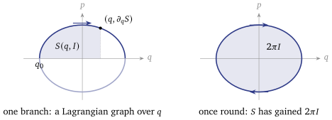
Theorem 6.5 (Action–angle coordinates sketched). Near $\Sigma$ there are functions $\varphi_1,\dots,\varphi_n$ , defined modulo $2\pi$ , such that $(\varphi,I)$ are canonical coordinates, $\symp=\sum_i\dd\varphi_i\wedge\dd I_i$ . In them $H=K(I)$ and $\dot I_i=0,\qquad \dot\varphi_i=\freq_i(I)=\frac{\partial K}{\partial I_i}.$ (6.4)

Sketch. Near a point of $\Sigma$ where the torus is a graph over $q$ , write it as $p=\sigma(q;I)$ . It is Lagrangian (Theorem 5.7), so $\sigma$ is closed (Proposition 4.14) and locally $\sigma=\dd_qS$ with $S(q,I)=\int_{q_0}^{q}p\cdot\dd q\qquad\text{(along the torus with actions }I).$ (6.5) Take $S$ as a type-2 generating function with new momenta $P=I$ . By Proposition 4.9 the new positions $\varphi_i=\partial S/\partial I_i$ make $(\varphi,I)$ canonical, and since the graph lies in the level set, $H(q,\partial S/\partial q)=K(I)$ : this $S$ solves Hamilton–Jacobi (4.7). Hamilton’s equations for $K(I)$ are (6.4).

$S$ is not a function on the torus. Continued once round $\gamma_j$ , it gains $\oint_{\gamma_j}p\cdot\dd q=2\pi I_j$ , by (6.1). So $\varphi_i=\partial S/\partial I_i$ gains $2\pi\,\partial I_j/\partial I_i=2\pi\delta_{ij}$ : the $\varphi_i$ are angles, defined modulo $2\pi$ , and round $\gamma_j$ only $\varphi_j$ turns. Where the torus is not a graph over $q$ — at turning points — one uses a mixed set of coordinates instead; that routine patching is what is omitted (Arnold, §50 C).

Figure 6.1. The generating function

S(q,I)

of (6.5) for a curve. Left:

S

is the shaded area under the upper branch. Right: once round the cycle it has gained

2\pi I

, which is why

\varphi=\partial S/\partial I

is an angle.

The practical route: separation of variables

In practice nobody computes the lattice first. If the Hamilton–Jacobi equation separates in some coordinates $q_1,\dots,q_n$ — if $S=\sum_iS_i(q_i)$ , so that on the level set each $p_i$ is a function of its own $q_i$ and of the constants $f$ only — then the torus is a product of closed curves $C_i$ in the separate $(q_i,p_i)$ -planes. Going once round $C_i$ with the other coordinates frozen is a cycle on the torus, and the actions are one-dimensional integrals, $I_i=\frac{1}{2\pi}\oint_{C_i}p_i\,\dd q_i .$ (6.6) The recipe for the rest of the lecture is: choose the cycle; integrate; invert to get $K(I)$ ; differentiate to get $\freq$ .

6.3 The harmonic oscillator

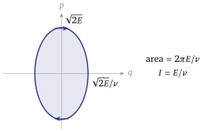
$H=\tfrac12(p^{2}+\freq^{2}q^{2})$ , the oscillator of Lecture 1. The level set at $E>0$ is an ellipse with semi-axes $\sqrt{2E}/\freq$ and $\sqrt{2E}$ , traversed clockwise. By Proposition 6.2 and the sign count of §3.4 the action along the motion is the enclosed area over $2\pi$ (Figure 6.2): $I=\frac{1}{2\pi}\,\pi\,\frac{\sqrt{2E}}{\freq}\sqrt{2E}=\frac{E}{\freq}, \qquad K(I)=\freq I,\qquad \frac{\dd K}{\dd I}=\freq .$ The angle: on the upper branch $S=\int^{q}\sqrt{2\freq I-\freq^{2}q^{2}}\,\dd q$ , so $\varphi=\partial S/\partial I=\arcsin\big(q\sqrt{\freq/2I}\big)$ , that is, $q=\sqrt{2I/\freq}\,\sin\varphi,\qquad p=\sqrt{2\freq I}\,\cos\varphi .$ The Jacobian of $(\varphi,I)\mapsto(q,p)$ is $\cos^{2}\varphi+\sin^{2}\varphi=1$ , so $\dd q\wedge\dd p=\dd\varphi\wedge\dd I$ : canonical, as Theorem 6.5 promised. This is the reference case: the frequency does not depend on the action. Lecture 1 observed that the oscillator’s period is the same on every ellipse; now we see that is the statement $K''(I)=0$ , and the pendulum breaks it.

Figure 6.2. The oscillator’s action is the area of its orbit over

2\pi

. The orbit runs clockwise, which makes it the negatively oriented boundary; with

\dd(p\cdot\dd q)=-\symp

the two signs cancel and

I>0

6.4 The pendulum, both regimes

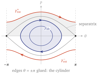
$H=\tfrac12p^{2}-\cos\theta$ on the cylinder $S^{1}\times\R$ ((1.2), (1.1)). With one degree of freedom every regular compact level-set component is a circle and the orbit itself is the cycle, so there is no choice of basis to make. The difficulty is different: the cycle is not the same kind of loop at every energy (Figure 6.3).

$-1<E<1$ , libration: one closed curve round $(0,0)$ . It bounds a disc on the cylinder, and $2\pi I$ is the area it encloses.
$E>1$ , rotation: two components, $p>0$ and $p<0$ , each going once round the cylinder. Neither bounds anything. Deforming the curve $p=\sqrt{2(E+\cos\theta)}$ down to the zero section $p=0$ , on which $p\,\dd\theta$ vanishes, sweeps out the strip beneath it, and $2\pi I$ is the area of that strip — the difference of the two integrals, by Stokes on the strip, both loops taken in the direction of motion. The branch $p<0$ is its mirror image and has the same action: it runs the other way round the cylinder with $p<0$ , so $p\,\dd\theta>0$ again.
$E=1$ is the separatrix, where the level set is not a circle, and $E=-1$ the equilibrium.

The two regimes cannot be merged into one formula: they integrate over loops of different kinds.

Figure 6.3. The pendulum’s two kinds of cycle on the unrolled cylinder (

\theta=\pm\pi

are one line; the dot there is the unstable equilibrium). Libration curves (indigo,

E=-0.5

0.3

) bound discs; rotation curves (red,

E=2

) bound nothing, and their action is the grey strip over

2\pi

The complete elliptic integrals

Both regimes lead to the same two integrals, and they are defined here, not assumed.

Definition 6.6 (Complete elliptic integrals). For $0\le k<1$ , the complete elliptic integrals of the first and second kind, in the modulus $k$ , are $\mathrm K(k)=\int_0^{\pi/2}\frac{\dd\psi}{\sqrt{1-k^{2}\sin^{2}\psi}}, \qquad \mathrm E(k)=\int_0^{\pi/2}\sqrt{1-k^{2}\sin^{2}\psi}\;\dd\psi .$ (6.7)

What we need about them: $\mathrm K(0)=\mathrm E(0)=\pi/2$ ; $\mathrm E(1)=1$ ; and as $k\to1$ , with $k'=\sqrt{1-k^{2}}$ , $\mathrm K(k)=\ln\frac{4}{k'}+o(1)$ (6.8) (cited: DLMF 19.12.1). $\mathrm K$ diverges because at $k=1$ the integrand becomes $1/\cos\psi$ .

Libration

Proposition 6.7 (The librating pendulum). For $-1<E<1$ put $k^{2}=(1+E)/2$ . Then $T=4\,\mathrm K(k),\qquad I=\frac{8}{\pi}\Big[\mathrm E(k)-(1-k^{2})\,\mathrm K(k)\Big].$ (6.9)

Proof. On the level set, $E+\cos\theta=E+1-2\sin^{2}(\theta/2) =2\big(k^{2}-\sin^{2}(\theta/2)\big)$ , so $p=2\sqrt{k^{2}-\sin^{2}(\theta/2)}$ on the upper branch, and the turning points are $\sin(\theta_0/2)=\pm k$ . Substitute $\sin(\theta/2)=k\sin\psi ,\qquad \psi\in[-\pi/2,\pi/2].$ (6.10) Then $p=2k\cos\psi$ and $\dd\theta=2k\cos\psi\,\dd\psi/\sqrt{1-k^{2}\sin^{2}\psi}$ , so $\dd\theta/p=\dd\psi/\sqrt{1-k^{2}\sin^{2}\psi}$ . The orbit is four copies of the quarter from $\theta=0$ to $\theta_0$ , and $T=\oint\dd\theta/\dot\theta=\oint\dd\theta/p$ , so $T=4\mathrm K(k)$ . For the action, the area is four times the area under the upper branch from $0$ to $\theta_0$ : $I=\frac{4}{2\pi}\int_0^{\theta_0}p\,\dd\theta =\frac{2}{\pi}\int_0^{\pi/2}\frac{4k^{2}\cos^{2}\psi}{\sqrt{1-k^{2}\sin^{2}\psi}}\,\dd\psi .$ Write $k^{2}\cos^{2}\psi=(1-k^{2}\sin^{2}\psi)-(1-k^{2})$ ; the integral splits into $\mathrm E(k)-(1-k^{2})\mathrm K(k)$ .

Rotation

Proposition 6.8 (The rotating pendulum). For $E>1$ put $k^{2}=2/(1+E)$ , again a modulus below $1$ . Then, on each of the two components (the derivation is an exercise: set $\psi=\theta/2$ and use $E+\cos\theta=(E+1)(1-k^{2}\sin^{2}\psi)$ ), $T=2k\,\mathrm K(k),\qquad I=\frac{4}{\pi k}\,\mathrm E(k),$ (6.11) where $T$ is the time for $\theta$ to advance by $2\pi$ .

The rotating pendulum at high energy

As $E\to\infty$ , $k\to0$ and $I\approx\sqrt{2E}$ , $T\approx2\pi/\sqrt{2E}$ : a free rotor with $p=\sqrt{2E}$ , which does not feel gravity. In both regimes the reader can differentiate (6.9) and (6.11) and find $\dd I/\dd E=T/2\pi$ , as Corollary 6.4 says it must.¹

The separatrix: where the torus degenerates

Figure 6.4. The pendulum’s action

I(E)

, from (6.9) and (6.11). Dotted: the oscillator of the pendulum’s small swings, frequency

1

and energy

E+1

measured from the bottom of the well, so

I=E+1

. At the separatrix it jumps, and its tangents are vertical, since

\dd I/\dd E=T/2\pi

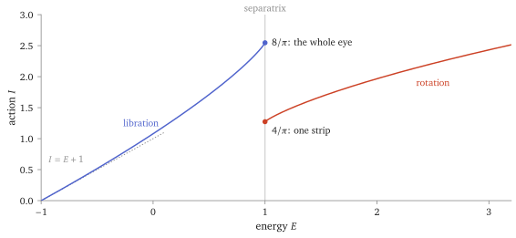
At $E=1$ the level set is the separatrix $p=\pm2\cos(\theta/2)$ : the unstable equilibrium $(\pi,0)$ , where $\dd H=0$ , and two orbits that leave it and return to it. It is not a circle, and Theorem 5.7 does not apply: hypothesis (I) fails at the equilibrium. Approaching it from either side the tori still exist, and two things happen to them. (A third, the jump of the action visible in Figure 6.4, is a reading at the end of this section.)

The period diverges, logarithmically (Figure 6.5). With (6.8): below, $k'^{2}=(1-E)/2$ and $T=4\mathrm K\approx4\ln(4/k')$ ; above, $k'^{2}=(E-1)/(E+1)\approx(E-1)/2$ and $T=2k\mathrm K\approx2\ln(4/k')$ . So $T=2\ln\frac{32}{1-E}+o(1)\quad(E\uparrow1),\qquad T=\ln\frac{32}{E-1}+o(1)\quad(E\downarrow1).$ (6.12) The coefficient on the rotation side is half the libration one. The reason is visible in Figure 6.3: almost all of the time is spent near the saddle, where the motion is slowest, and a libration loop passes near it twice per period — at $\theta\approx\pi$ and at $\theta\approx-\pi$ , which on the cylinder are the same point — while a rotation loop passes once.

The frequency goes to zero. $\freq=2\pi/T\to0$ : the torus degenerates into a set on which the motion takes infinitely long to go round.

Figure 6.5. The pendulum’s period

T(E)

, from (6.9) and (6.11), with the separatrix asymptotics (6.12) dashed. It starts at the oscillator’s

2\pi

(dotted) and diverges on both sides of

E=1

, twice as fast from below as from above.

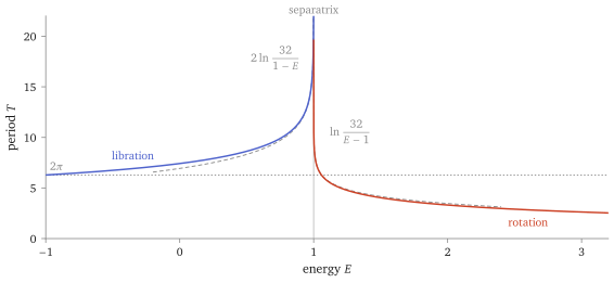
The action jumps (Figure 6.4). As $E\uparrow1$ , $k\to1$ and $I\to8/\pi$ , which is $1/2\pi$ times the area of the eye, $\int_{-\pi}^{\pi}4\cos(\theta/2)\,\dd\theta=16$ . As $E\downarrow1$ , $I\to4/\pi$ , one strip of area $8$ . One libration torus becomes two rotation tori, and the area is shared between them. The function $I$ is not continuous across the separatrix because the cycle is not.

Why a logarithm. Near the saddle put $\theta=\pi+x$ . Then $H\approx\tfrac12p^{2}-\tfrac12x^{2}+1$ , the inverted oscillator, whose orbits are the hyperbolas $p^{2}-x^{2}=2(E-1)$ . The time to cross a fixed box $\abs{x}\le\delta$ along the hyperbola is $\int\dd x/\sqrt{x^{2}+2(E-1)}\approx\ln\big(\delta^{2}/\abs{E-1}\big)$ , which diverges like $\ln(1/\abs{E-1})$ ; the time spent outside the box stays bounded. One crossing per rotation, two per libration — the factor $2$ in (6.12). The constant $32$ needs the exact integral: it is where (6.8) is used.

6.5 Quasi-periodic motion and resonance

The theorem says the motion is a straight line on a torus. It does not say the motion is periodic, and the difference is the subject of Lecture 7.

Definition 6.9 (Resonance). A frequency vector $\freq\in\R^{n}$ is resonant if $k\cdot\freq=0$ for some nonzero $k\in\Z^{n}$ , and non-resonant otherwise. A torus is resonant if its frequency vector is.

A change of lattice basis replaces $\freq$ by $B\freq$ with $B$ an integer matrix of determinant $\pm1$ , and $k\cdot\freq=0$ becomes $(B^{-\mathsf T}k)\cdot(B\freq)=0$ : resonance is a property of the torus, not of the basis. For $n=2$ it says exactly that $\freq_1/\freq_2$ is rational (or a frequency vanishes).

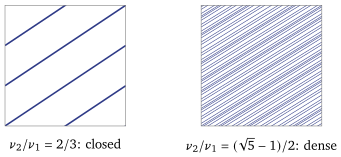
Proposition 6.10 (Winding on $T^{2}$ ). Let $\varphi(t)=\varphi(0)+\freq t$ on $T^{2}$ with $\freq_2\ne0$ . If $\freq_1/\freq_2$ is rational every orbit is closed; if it is irrational every orbit is dense.

Proof (★). Watch the orbit cross the circle $\varphi_2=0$ . It returns every $2\pi/\freq_2$ , having advanced $\varphi_1$ by $2\pi\alpha$ , $\alpha=\freq_1/\freq_2$ ; so the crossings are $\varphi_1^{(m)}=\varphi_1^{(0)}+2\pi m\alpha$ mod $2\pi$ . If $\alpha=a/b$ in lowest terms, the $b$ -th crossing is the first, and the orbit closes. If $\alpha$ is irrational the crossings are all distinct (else $m\alpha\in\Z$ for some $m\ne0$ ). Of any $N+1$ of them, two lie within $2\pi/N$ of each other on the circle; if they are crossings $m$ and $m+d$ , then every $d$ returns rotate the circle by a nonzero angle smaller than $2\pi/N$ , and iterating that rotation lands within $2\pi/N$ of any given point. So the crossings are dense in the circle. Every point of $T^{2}$ is reached from the circle by flowing for a time less than $2\pi/\abs{\freq_2}$ , and flowing for a fixed time is continuous, so the orbit is dense in $T^{2}$ .

For general $n$ the same holds: a non-resonant orbit is dense in $T^{n}$ , and with exactly $r$ independent integer relations $k\cdot\freq=0$ the closure of every orbit is a torus of dimension $n-r$ (cited: Arnold, §51 B and §51 D). So a torus is not an orbit: on a non-resonant torus a single trajectory visits every neighbourhood and never returns exactly, and only when $r=n-1$ (and $\freq\ne0$ ) is the torus foliated by closed orbits (Figure 6.6).

Figure 6.6. Straight-line motion on

T^{2}

, drawn on the square

[0,2\pi]^{2}

with opposite sides identified. Left: a rational ratio; the orbit closes after three turns of

\varphi_1

. Right: the golden ratio, drawn over a long but finite time; continued forever the orbit comes arbitrarily close to every point and never closes (Proposition 6.10).

In the oscillator every torus has the same $\freq=(\freq_1,\freq_2)$ , so they are all resonant or all not. That is special. Generically $\freq$ depends on $f$ , resonant and non-resonant tori are interleaved, and Lecture 7 asks which of them survive a perturbation.

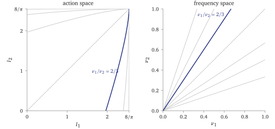
The other side of the coin is the frequency map. Call an integrable system non-degenerate if $I\mapsto\freq(I)$ is a local diffeomorphism, $\det(\partial^{2}K/\partial I^{2})\ne0$ . For $n\ge2$ the resonant tori, the preimages of the rational directions, are then dense but form a set of measure zero (Figure 6.7); for $n=1$ resonance means $\freq=0$ , and there may be none at all. Lecture 7 needs exactly this picture. Kepler, in the reading at the end of this lecture, is as degenerate as possible: its frequency map has rank one, and every torus is resonant.

Figure 6.7. The frequency map of two uncoupled librating pendula,

K=K_{\mathrm{pend}}(I_1)+K_{\mathrm{pend}}(I_2)

, computed from (6.9). It is non-degenerate:

\freq(I)

falls strictly from

1

I=0

0

at the separatrix

I=8/\pi

. The resonant tori

\freq_1/\freq_2=a/b

are lines through

0

in frequency space and curves in action space; one is marked.

6.6 What it buys

Free motion in the right variables. In $(\varphi,I)$ the motion is $\dot I=0$ , $\dot\varphi=\partial K/\partial I$ (Theorem 6.5): the first of the course’s five ideas, P1, made precise near one torus.
Frequencies from energies. $\freq=\partial K/\partial I$ (Corollary 6.4), and with one degree of freedom $T=2\pi\,\dd I/\dd E$ . The pendulum’s period follows from its action, and diverges at the separatrix.
The picture Lecture 7 perturbs. A non-degenerate frequency map makes the resonant tori dense and of measure zero, and Lecture 7 asks which tori survive a small perturbation.

6.7 Caveats, in one place

Status. The standing assumption about the neighbouring tori is cited (Arnold, §50 A). Proposition 6.2 is proved modulo Stokes. Theorem 6.5 is sketched, with the patching at turning points omitted. The rotating pendulum’s formulas (6.11) are stated, with their derivation an exercise, and the asymptotics (6.8) and the general- $n$ density of non-resonant orbits are cited. Proposition 6.3, Corollary 6.4 and Proposition 6.7 are proved; the proof of Proposition 6.10 is in a reading.
The choice of cycles. A different basis of the period lattice gives different actions, related by an integer matrix of determinant $\pm1$ (a reading). The motion, and whether a torus is resonant, do not change.
Local, not global. Action–angle variables are built near one torus. They break down where the tori degenerate, as at the pendulum’s separatrix, and they need not exist globally (optional lecture A).

6.8 Kepler, and superintegrability

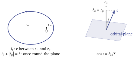
A particle in $\R^{3}\setminus\{0\}$ with $H=\tfrac12\abs{p}^{2}-\alpha/\abs{q}$ , $\alpha>0$ . In spherical coordinates $(r,\theta,\phi)$ — $\theta$ the polar angle, not the pendulum’s, and $\phi$ the azimuth, to be told apart from the angle variables $\varphi$ — $H=\frac12\Big(p_r^{2}+\frac{p_\theta^{2}}{r^{2}}+\frac{p_\phi^{2}}{r^{2}\sin^{2}\theta}\Big)-\frac{\alpha}{r}.$ (6.13) This is a central force, integrable with $F=(H,\abs{\ell}^{2},\ell_3)$ (Example 5.6), and in these coordinates $\ell_3=p_\phi,\qquad \abs{\ell}^{2}=p_\theta^{2}+\frac{p_\phi^{2}}{\sin^{2}\theta}.$ Write $\ell=\abs{\ell}$ . Fix $E<0$ and $0<\abs{\ell_3}<\ell<\alpha/\sqrt{-2E}$ (the last so that the radial motion is not a circle). On the level set $p_\phi=\ell_3,\qquad p_\theta=\pm\sqrt{\ell^{2}-\frac{\ell_3^{2}}{\sin^{2}\theta}},\qquad p_r=\pm\sqrt{2E+\frac{2\alpha}{r}-\frac{\ell^{2}}{r^{2}}},$ (6.14) and each momentum depends only on its own coordinate: Hamilton–Jacobi separates, $S=S_r(r)+S_\theta(\theta)+\ell_3\phi$ . The torus is a product of three circles — $r$ oscillating between the roots $r_-<r_+$ of $p_r=0$ , $\theta$ between the roots of $p_\theta=0$ , and $\phi$ going round — and (6.6) gives three actions (Figure 6.8): $I_\phi=\frac1{2\pi}\oint p_\phi\,\dd\phi=\ell_3,\qquad I_\theta=\frac1{2\pi}\oint p_\theta\,\dd\theta=\ell-\abs{\ell_3},\qquad I_r=\frac1{2\pi}\oint p_r\,\dd r .$ The first is immediate. The second is a one-variable integral of the same kind as the next one; it is an exercise, and we use it as stated.

Proposition 6.11 (The radial action). $\displaystyle I_r=\frac{\alpha}{\sqrt{-2E}}-\ell$ .

Proof. $I_r=\frac1\pi\int_{r_-}^{r_+}p_r\,\dd r$ , the loop being twice the passage from $r_-$ to $r_+$ . Differentiate in $\ell$ under the integral. This is legitimate: with $r=c-h\cos s$ , $c=\tfrac12(r_++r_-)$ , $h=\tfrac12(r_+-r_-)$ , the limits become $0$ and $\pi$ and the integrand becomes $\sqrt{-2E}\,h^{2}\sin^{2}s/r$ , smooth in $(s,\ell)$ ; transforming back gives $\frac{\partial I_r}{\partial\ell}=-\frac{\ell}{\pi}\int_{r_-}^{r_+}\frac{\dd r}{r^{2}p_r} =-\frac{\ell}{\pi}\int_{u_-}^{u_+}\frac{\dd u}{\sqrt{2E+2\alpha u-\ell^{2}u^{2}}}, \qquad u=\frac1r .$ The quadratic under the root is $\ell^{2}(u_+-u)(u-u_-)$ , and $\int_{u_-}^{u_+}\dd u/\sqrt{(u_+-u)(u-u_-)}=\pi$ (substitute $u=\tfrac12(u_++u_-)-\tfrac12(u_+-u_-)\cos s$ , and the integrand becomes $\dd s$ ). So $\partial I_r/\partial\ell=-1$ and $I_r=c(E)-\ell$ . To find $c(E)$ , let $\ell$ increase to the circular orbit, where $r_-=r_+$ : the interval of integration shrinks to a point with $p_r$ bounded, so $I_r\to0$ . The two roots of $2Er^{2}+2\alpha r-\ell^{2}=0$ coincide when $\alpha^{2}+2E\ell^{2}=0$ , i.e. $\ell=\alpha/\sqrt{-2E}$ . Hence $c(E)=\alpha/\sqrt{-2E}$ .

Figure 6.8. Kepler’s three actions.

I_r

is the radial oscillation between pericentre and apocentre;

I_\theta+\abs{I_\phi}=\ell

is the angular momentum;

I_\phi=\ell_3

its component along

e_3

, fixing the inclination

\iota

of the orbital plane.

Adding the three actions, $I_r+I_\theta+\abs{I_\phi}=\alpha/\sqrt{-2E}$ , so $K(I)=-\frac{\alpha^{2}}{2\big(I_r+I_\theta+\abs{I_\phi}\big)^{2}} .$ (6.15) The energy depends on the actions only through their sum. By (6.3), with $\mathcal J=I_r+I_\theta+\abs{I_\phi}$ , $\freq_r=\freq_\theta=\abs{\freq_\phi}=\frac{\alpha^{2}}{\mathcal J^{3}}$ (6.16) (with $\freq_\phi$ of the sign of $I_\phi$ ). All three frequencies are equal: every torus is resonant, in the sense of Definition 6.9, as resonant as it can be. The radial oscillation, the swing in $\theta$ and the turn in $\phi$ all close at the same moment, so every bounded Kepler orbit with $\ell\ne0$ is closed: $\varphi(t)=\varphi(0)+\freq(1,1,\pm1)\,t$ returns to its start after $2\pi/\freq$ . (The tori excluded above, $\ell_3=0$ or $\abs{\ell_3}=\ell$ , differ only in the choice of polar axis, and the same holds there; circular orbits are closed anyway. A bounded orbit with $\ell=0$ is radial and falls into the centre in finite time.) The common period is $T=2\pi\mathcal J^{3}/\alpha^{2}$ ; with the semi-major axis $a=\tfrac12(r_-+r_+)=\alpha/(-2E)$ this is $T=2\pi a^{3/2}/\sqrt\alpha$ , Kepler’s third law.

In celestial mechanics the actions are taken as $(\mathcal J,\ell,\ell_3)$ — the Delaunay variables — whose conjugate angles are the mean anomaly, the argument of pericentre and the longitude of the node. Since $K$ depends on $\mathcal J$ alone, only the first angle moves. We name them and do not use them.

What a perturbation breaks

Add a small $\beta/r^{2}$ to the potential. It only replaces $\ell^{2}$ by $\ell^{2}+2\beta$ in $p_r$ , so the proof of Proposition 6.11 goes through unchanged and $I_r=\frac{\alpha}{\sqrt{-2E}}-\sqrt{\ell^{2}+2\beta},\qquad K=-\frac{\alpha^{2}}{2\big(I_r+\sqrt{\ell^{2}+2\beta}\big)^{2}} .$ The motion is still in a plane, and $\ell$ is the action of the angle in it. Now $\partial K/\partial\ell=\freq_r\,\ell/\sqrt{\ell^{2}+2\beta}$ : the angular frequency differs from the radial one. In one radial period the orbit turns by $2\pi\ell/\sqrt{\ell^{2}+2\beta}$ , not $2\pi$ , so the pericentre moves on every pass, and unless the ratio is rational the orbit never closes; it fills the annulus $r_-\le r\le r_+$ densely (Arnold, §8 C) (Figure 6.9). The degeneracy (6.16) is the whole reason Kepler orbits close, and it is fragile.

Figure 6.9. Five radial periods, with the same

\alpha

\ell

and

e

. Left, Kepler: the radial and angular frequencies are equal and the ellipse retraces itself. Right, with

\beta/r^{2}

added (

\beta=0.12

\ell=1

): the angle between successive pericentres (dots) is

2\pi\ell/\sqrt{\ell^{2}+2\beta}<2\pi

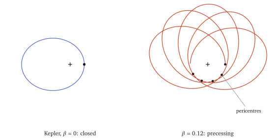
. Both curves are exact orbits (scripts/figures/kepler_precession.py).

6.9 Superintegrability and Laplace–Runge–Lenz

Equal frequencies are the footprint of extra integrals. For Kepler the extra one is the Laplace–Runge–Lenz vector $A=p\times\ell-\alpha\,\frac{q}{\abs{q}} .$ (6.17) It is conserved, $\pb{A_i}{H}=0$ (an exercise); it lies in the orbital plane, $\ell\cdot A=0$ ; and it points from the centre to the pericentre, with length $\abs{A}=\alpha e$ (Figure 6.10). A conserved vector pointing at the pericentre is exactly the statement that the pericentre does not move.

Figure 6.10. The Laplace–Runge–Lenz vector on an orbit with

\alpha=\ell=1

e=0.6

. At

q

the two terms of (6.17), drawn to scale, add to the same

A

as at the pericentre.

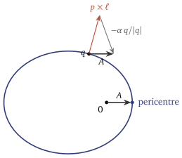
Count the integrals. $H$ , the three $\ell_i$ and the three $A_i$ are seven functions on a six-dimensional phase space, tied by two relations, $\ell\cdot A=0,\qquad \abs{A}^{2}=\alpha^{2}+2H\,\abs{\ell}^{2},$ and $5$ of them are independent. The Jacobian has rank $5$ at one sample point,² so some $5\times5$ minor is not identically zero; the minors are real-analytic on the connected set $q\ne0$ , and such a function vanishing on an open set vanishes identically, so the minor is nonzero on a dense open set.

Definition 6.12 (Superintegrable). An integrable system with $n$ degrees of freedom is superintegrable if it has more than $n$ independent first integrals, and maximally superintegrable if it has $2n-1$ .

Kepler is maximally superintegrable: $5=2\cdot3-1$ . The oscillator with equal frequencies is the other standard example.

The extra integrals explain the closed orbits a second way. Fix $E<0$ and $\ell\ne0$ . Then $\ell$ fixes the orbital plane and the sense of motion, $A$ the eccentricity $e=\abs{A}/\alpha$ and, if $e>0$ , the direction of the pericentre, and $H$ the size: one ellipse in $q$ -space. Over each of its points $p$ is fixed as well, by $p=\ell\times(A+\alpha q/\abs{q})/\abs{\ell}^{2}$ , which inverts (6.17) because $p\perp\ell$ . So the joint level set of $(H,\ell,A)$ is a single closed curve in phase space. $\hvf{H}$ does not vanish on it ( $p\ne0$ since $\ell\ne0$ ), so the orbit is the whole curve and is periodic. The integrals do not all commute: $\pb{\ell_i}{A_j}=\sum_k\epsilon_{ijk}A_k$ and $\pb{A_i}{A_j}=-2H\sum_k\epsilon_{ijk}\ell_k$ (an exercise), so at most $n=3$ of them can be the integrals of Theorem 5.7 at once.

Which central potentials share Kepler’s luck? Bertrand’s theorem: among smooth central potentials that have bounded orbits at all, the only ones all of whose bounded non-collision orbits are closed are, up to an additive constant, $-\alpha/r$ with $\alpha>0$ and $\tfrac12\freq^{2}r^{2}$ (cited: Arnold, §8 D, through a sequence of problems).

6.10 Bridge to Part II: Bohr–Sommerfeld

The old quantum theory quantised the actions, $\oint_{\gamma_i}p\cdot\dd q=2\pi\hbar\,n_i,\qquad n_i\in\Z, \qquad\text{that is,}\qquad I_i=\hbar\,n_i .$ (6.18) For the oscillator it gives $E=\hbar\freq n$ , which misses the zero-point energy $\tfrac12\hbar\freq$ ; for Kepler, (6.15) with $\mathcal J=\hbar n$ , $n=1,2,\dots$ , gives $E=-\alpha^{2}/2\hbar^{2}n^{2}$ , the Bohr levels. The correction $n\mapsto n+\tfrac12$ at each turning-point cycle, and the reason (6.18) works as well as it does, belong to Part II. What matters now is its shape: quantisation is a condition on the actions, and Lecture 10 will find the Bethe equations to be this condition for a many-body system.

Summary

Actions: $I_i=\frac1{2\pi}\oint_{\gamma_i}p\cdot\dd q$ , well defined because $p\cdot\dd q$ is closed on the torus (Proposition 6.2); their derivatives are the periods (Proposition 6.3), and $\freq=\partial K/\partial I$ (Corollary 6.4).
Angles: from the generating function $S(q,I)=\int p\cdot\dd q$ , which gains $2\pi I_j$ round $\gamma_j$ (Theorem 6.5).
The oscillator: $I=E/\freq$ , with a frequency that does not depend on the action. The librating pendulum: $T=4\,\mathrm K(k)$ and $I=\frac8\pi\big[\mathrm E(k)-(1-k^{2})\mathrm K(k)\big]$ , with the period diverging at the separatrix (6.12).
A torus is not an orbit: rational frequency ratios give closed orbits, irrational ones dense orbits (Proposition 6.10), and a non-degenerate frequency map interleaves the two.
Next: Lecture 7 asks what happens to all this when the system is perturbed, and meets chaos.

Worked in the tutorial: Exercise Sheet 6.

References

Arnold, Mathematical Methods of Classical Mechanics, §50 (action–angle variables: the construction and the neighbourhood statement), §51 (conditionally periodic motion) and §8 (central fields, Bertrand’s theorem); Babelon, Bernard and Talon, Introduction to Classical Integrable Systems, ch. 2; DLMF, §§19.2 and 19.12 (complete elliptic integrals and their behaviour as $k\to1$ ). Conventions. Arnold writes $\symp=\sum\dd p\wedge\dd q$ , the negative of ours; his actions come out positive for the same reason ours do (§3.4).

The whole bibliography, lecture by lecture →

scripts/check-l5-pendulum.py, check 2 — a numerical check at four energies, not a proof; the proof is Proposition 6.3.↩︎
scripts/check-l5-algebra.py, check 7: the relations symbolically, the rank exactly at a rational sample point.↩︎