10.1 The question
Part I found a classical many-body system’s conserved quantities as the traces of one matrix, commuting because of one local identity. Part II builds the quantum counterpart: Lecture 14 constructs commuting operators as the traces of one matrix again, and Lecture 15 obtains the chain’s Hamiltonian from their logarithmic derivative and diagonalises them. The classical count does not carry over, since for a finite quantum chain counting commuting operators decides nothing (Lecture 0’s caveat). It starts, as the subject did, with an exact solution found by a guess. So the question of this lecture is
how do you find the exact eigenstates of an interacting spin chain?
The answer is Bethe’s ansatz: plane waves of flipped spins, whose only interaction is a two-body phase (Proposition 10.1), quantised by the Bethe equations (Theorem 10.2). The rule for passing from Part I to Part II comes first.
The rule of translation
Quantum mechanics keeps the shape of the classical equation of motion and changes its ingredients. States are vectors in a Hilbert space, observables are Hermitian operators, and in the Heisenberg picture an observable evolves by (10.1) Set against , this is the substitution — checked on the one bracket that fixes it, against . An operator is conserved exactly when , and two conserved operators are “in involution” when they commute. From here on , except in Lecture 14, where the classical limit is taken and is written.
10.2 The model
The spin- Heisenberg chain on a ring of sites is (10.2) with the permutation of the spins on sites and (Definition 9.4). On the basis of up and down spins the bond term is simple: gives zero on a parallel pair, and on an antiparallel pair it returns times (the swapped pair minus the pair itself).
Symmetries. The total spin commutes with every , since exchanging two spins does not change their sum; so commutes with — the symmetry — and with the shift that moves every spin one site on. , where is the number of down spins, so does not mix different .
The reference state. In every bond is parallel, so . Since has eigenvalues , each bond term has eigenvalues and . The sign of decides what is. For every bond term is , so and is a ground state: the ferromagnet, and the intuition of this lecture, where flipped spins are excitations that cost energy. For , the antiferromagnet and the course’s frozen convention, is the highest level; for even the ground state lies at (Lecture 16); for odd the lowest level is made of spin- multiplets — two of them for (the check script) — with highest weights at . Every formula below holds for either sign.
What must be found. Because commutes with , its eigenspaces are sums of multiplets, and each multiplet of total spin contains exactly one highest-weight vector, killed by , with ; the rest of the multiplet is got from it by applying . Decomposing (a prerequisite), the multiplets of spin number (10.3) So the task is: find the highest-weight eigenvectors with down spins, for each . The method looks for them as waves of flipped spins.
10.3 One magnon
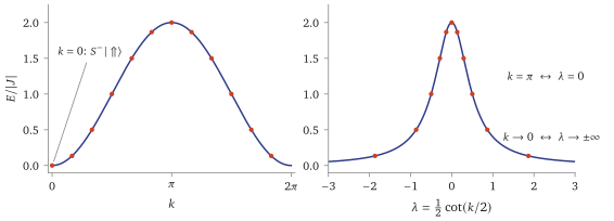
Let be the state with one down spin, at site . Of the bonds only the two touching are antiparallel, so (10.4) a particle hopping on a ring. The plane wave is an eigenvector with (10.5) This is a magnon, or spin wave: one flipped spin spread over the ring with momentum . For the ferromagnet, at small : a quasiparticle with a quadratic dispersion.
Which are highest weight? , which vanishes for and not for . And is : not a new state, but the ferromagnetic multiplet one step down. So the magnons with are the highest-weight states with , as (10.3) says.
The rapidity
From now on the momentum is traded for a rapidity , (10.6) It maps onto the real line, to , and to . The reason for the change appears in the next section: the two-magnon phase depends on and in a complicated way, but on and only through their difference. Three names for one number — , and — are a standard place to get lost; the lecture fixes here and keeps it.
10.4 Two magnons
The equations
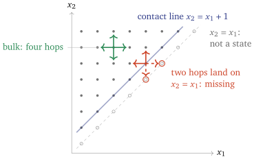
Let , , have down spins at and , and look for an eigenvector whose amplitude on is . For the moment think of a long open line and ignore the ends; the ring enters at the end of this section. There are two cases: (10.7) (10.8) In the bulk each down spin hops independently, with four antiparallel bonds. When the two are neighbours the bond between them is parallel: neither can hop onto the other, and there are only two antiparallel bonds (Figure 10.1).
Bethe’s ansatz and the contact condition
Two far-apart magnons should move as two plane waves, so try (10.9) the two momenta, carried in either order. Each term solves the bulk equation (10.7) with the same energy (10.10) because in the bulk the two coordinates hop independently. The formula (10.9) defines on the whole plane, the diagonal included, and satisfies the right-hand side of (10.7) at every point. Compare (10.8) with (10.7) evaluated at : the two differ by exactly the two missing hops, and the extra diagonal term, So the ansatz solves the true equations if and only if the contact condition (10.11) holds. It concerns values of at configurations that do not exist; that is the point of the trick.
Proposition 10.1 (The two-magnon S-matrix). The ansatz (10.9) satisfies the contact condition if and only if (10.12) with the rapidities (10.6) of ; at , the pole of , read it as .
Proof. Substitute: every term of (10.11) carries , and with what remains is Now put and clear the denominators : the first bracket becomes , and the second is the same with , namely . Divide.
Three properties of carry the rest of the lecture. It depends on the rapidities only through , which is why rapidities were introduced. For real it is a phase, , and . And : with equal rapidities and , so the Bethe vector is zero — a Pauli principle that was not put in. (Whether a rescaled limit could still give a state belongs to the completeness question, a reading; roots are taken pairwise distinct from now on.) Physically, the two magnons meet, and the outgoing wave carries the same two momenta, exchanged, times a phase: no reflection into new momenta, and is the entire effect of the collision. For two classical particles of equal mass that is forced by energy and momentum conservation (Proposition 0.1); for magnons it is not, at least at total momentum , where is however is split. Non-diffraction here is found by the ansatz, not supplied by kinematics.
The ring
On the ring, with is the same state as the down spins at and . Extend by requiring (10.13) then the equations of the ring are the equations of the line for , including the pair adjacent across the seam, , . Substituting (10.9) and matching the coefficients of the two plane waves gives and . With Proposition 10.1 these are the Bethe equations for two magnons; the reading at the end of the lecture states them as a theorem, and §10.5 does magnons at once.
10.5 magnons
For down spins at , Bethe’s ansatz is a sum over all ways of handing out the momenta: (10.14) where “ puts before ” means ; , and for this is (10.12). The amplitude collects one factor of for each pair of magnons whose momenta have been exchanged.
Theorem 10.2 (Bethe 1931 sketched). Let be finite and pairwise distinct, none equal to , no two differing by , and let them satisfy the Bethe equations (10.15) Then (10.14), if it is not the zero vector, is an eigenvector of with (10.16)
Sketch. Bulk. If no two down spins are neighbours, each plane wave describes independent hoppers, and the energies add. One contact. If and no other pair touches, the true equation differs from the extended bulk equation by times the contact expression (10.11) in the coordinates , the others held fixed. Pair each with , which exchanges the momenta in positions and . Their two terms are a two-magnon wave in times a common factor, so by Proposition 10.1 they cancel in the contact expression if — and the product in (10.14) is built to do exactly that, gaining or losing the one factor for the pair exchanged (using ). Several contacts. is a sum of bonds; each missing hop belongs to one adjacent pair, so the true equation differs from the extended one by a sum of contact expressions, one per adjacent pair, each vanishing as before. A block of three neighbours needs nothing new. (The check script verifies the case symbolically, three neighbours included.) Periodicity. The ring’s condition is . In the right-hand side the term of is the plane wave in which carries , , followed by the others in the order of ; call that ordering . So the condition reads . Passing from to moves from last to first, past every other magnon once: each pair changes its order, and by (10.14) . The condition is therefore , which is (10.15).
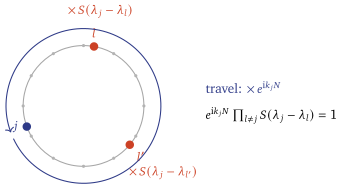
Reading the Bethe equations. Write (10.15) as (10.17) Carry magnon once round the ring: it picks up from the distance travelled and one factor from each other magnon it passes, and it must come back to the same wavefunction (Figure 10.2). The many-body problem has become coupled equations for numbers.
10.6 The logarithmic form
For real let , so that . Taking logarithms of (10.15) for real rapidities, (10.18) the signs and having gone into : the Bethe quantum numbers are integers if is odd and half-odd integers if is even. Summing (10.18) over (the ’s cancel in pairs, being odd) and using gives the momentum (10.19) As the left side of (10.18) tends to , so belongs to a root at infinity. The finite real roots of every solution met here have , which leaves values (the limit explains the endpoint, not the bound). For at and , where every solution is known, each choice of two distinct values gives exactly one real solution and there are no others — of them; at , , each of the choices gives one (the check script; not proved in general). The label states the way occupation numbers label free fermions. The tutorial at the end of this lecture draws them as the crossings of a counting function, the picture Lecture 16 takes to .
Rewrite (10.17) with : (10.20) The collects the minus signs of . With one magnon the sum is empty and (10.20) is : exactly the Bohr–Sommerfeld condition of a particle going once round a ring of circumference (a reading of Lecture 6), and here it is not an approximation but the exact spectrum (10.5).
Highest weight
Theorem 10.3 (Bethe vectors are highest weight cited). Under the hypotheses of Theorem 10.2, if the vector (10.14) is not zero it is a highest-weight vector: . Consequently .
For this is the computation of §10.3: is , zero on the grid unless , i.e. unless . In general is a sum of -magnon plane waves whose coefficients are, term by term, combinations of the Bethe equations, so vanish on solutions (Faddeev and Takhtajan 1981). The consequence follows because a highest-weight vector has .
10.7 What it buys
Exact eigenstates of an interacting chain, labelled by rapidities that solve coupled equations (Theorem 10.2), with energy and momentum read off them (10.16).
Scattering that only exchanges momenta. The whole effect of a collision is the phase , and the -magnon state is built from it alone: the second face of integrability that Lecture 0 described, now for a quantum system.
Quantum numbers. In logarithmic form each real root carries a quantum number (10.18), as occupation numbers label free fermions; Lecture 16 takes them to as a density.
10.8 Caveats, in one place
Status. Proposition 10.1 is proved and Theorem 10.2 is sketched, its contact bookkeeping routine. That Bethe vectors are highest weight (Theorem 10.3) is cited.
Completeness. Whether every highest-weight state is a Bethe state is not proved here. At , all nine are found, six from real roots and three from complex or singular ones (the tutorial and the reading).
Real quantum numbers. That each allowed set of distinct gives a real solution is checked here only in small cases, not proved in general. At and with , where every solution is known, each set gives exactly one; at with each of the ten sets gives one, and uniqueness is not checked.
The hypotheses of Theorem 10.2 — finite, pairwise distinct rapidities, none equal to , no two differing by — exclude the singular solutions, which the reading treats.
An analogy, not a limit. At the Bethe equation is Bohr–Sommerfeld; with magnons the resemblance is structural. No is taken, and magnons have no classical phase space.
10.9 A worked check, and how to reproduce it
| quantum numbers | roots | |||
|---|---|---|---|---|
| real | ||||
| real | ||||
| real | / | / mirror | ||
| real | / | / mirror | ||
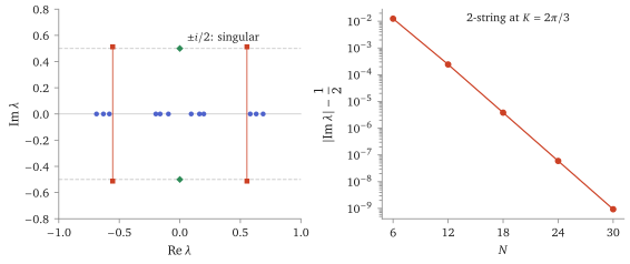
| 2-string | — | |||
| singular | — | , regularised |
Table 10.1 and Figure 10.3 are the lecture checked end to end on the smallest interesting case. The Bethe solutions, and the eigenvectors of on the states with two down spins that are killed by , agree in both directions, with every type of solution present (the tutorial says how to reproduce this). At they agree again: real solutions, strings and the singular pair make the highest-weight states (the check script). The same script finds the ground state of the whole antiferromagnet as the Bethe state with and , all real: the state Lecture 16 takes to .
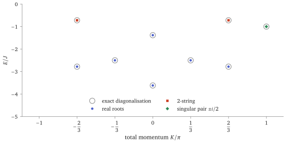
scripts/figures/xxx_bethe.py) matches the two lists, energy and momentum, to in both directions.
Reproducing the check. For every solution can be found, not just the real ones. At each total momentum , write and clear denominators in the first equation of (10.22): it becomes a polynomial of degree at most in (the degree drops at ), with the roots (the singular pair, whose partner is infinite) and (a root at infinity, a descendant). Discard both from the search for regular roots, and keep the others whose two rapidities are finite and distinct; for even add the singular state by hand (for odd , and , there is none). Separately, diagonalise on the states with two down spins and keep the eigenvectors killed by , sorted by momentum. At this is Table 10.1.
Roots and holes. Define the counting function (10.21) The roots are the points where passes one of its values ; the allowed values it passes where there is no root are holes (Figure 10.4). In Lecture 16, where , the densities of roots and of holes add up to , and the ground state and its excitations are read off this picture.
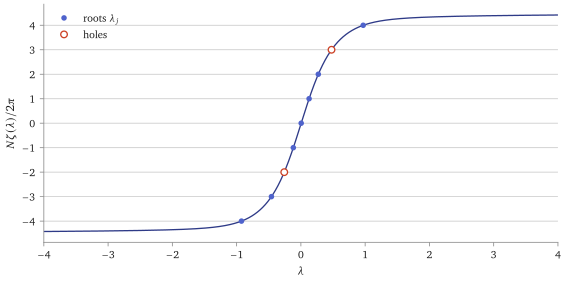
scripts/figures/xxx_bethe.py, which asserts the equations to and that the curve increases.)The singular pair, regularised. Put and , with . Then and , while . In the first equation of (10.22) the left side is and the right side , so . In the second the left side is and the right side , so . The two agree if and only if , that is, even. With that , in (10.9) the first wave is of order on nearest neighbours and smaller elsewhere, and the second, whose amplitude is of order , contributes at order only to the pair adjacent across the seam; divided by , the vector tends to a multiple of (the check script does this to 400 digits for ). The energy is finite: , the two infinities cancelling.
10.10 Two magnons as a theorem; descendants; complex and singular roots
Theorem 10.4 (Two magnons). Let be finite, neither equal to , with , and suppose (10.22) Then (10.9) with (10.12), if it is not the zero vector, is an eigenvector of with , , and momentum : .
Proof. By Proposition 10.1 and the reduction above, the ansatz solves the equations of the line; by (10.13) it solves those of the ring provided and , which are (10.22). The energy is (10.10) in rapidities, and the momentum is read off the plane waves.
Nothing here needed real. Multiplying the two equations gives : the total momentum is quantised as for one particle, and all the interaction sits in the relative motion.
The periodicity step is a complete argument; what the sketch leaves out is the bookkeeping of the contact steps, which is routine. One step deserves a flag. The amplitudes were defined by a closed formula, so they are consistent automatically; had we only known the two-body rule , we would have had to check that different sequences of exchanges leading to the same agree. For numbers that commute this is free. For particles carrying an internal label, becomes a matrix, and the same requirement becomes the Yang–Baxter equation — Lecture 13’s subject.
The descendants need no new solutions, and one of them is a root at infinity. If then , , and (10.9) becomes : exactly applied to the one-magnon state , since adds the second down spin at every other site. The equation for becomes the one-magnon condition . So the states of a multiplet below its top are applied, repeatedly, to its highest-weight vector — one application being literally a Bethe state with one root at infinity — and (10.3) is the number of finite-root Bethe states the method must find. Whether it always finds them is the completeness question below.
For and , (10.3) asks for highest-weight states, and real roots supply . The other three are two strings and one singular solution.
Strings
Suppose . Then is nearer to than to , so and the left side of (10.15) grows like . For large the right side must follow, and it can only do so through a nearly vanishing denominator: some with . The argument is heuristic (it assumes stays away from as grows); for at fixed total momentum it suggests (10.23) a 2-string. In the wavefunction (10.9), , so the wave grows with ; but its amplitude tends to zero as . What remains, , decays in : a bound state of two magnons. For the exact string , and for the ferromagnet this lies below the two-magnon continuum at the same , whose bottom is , by : two flipped spins side by side cost two broken bonds, two apart cost four. Figure 10.5 shows the roots of and the decay of .
scripts/figures/xxx_bethe.py.)For larger the same argument makes complex roots cluster into strings of any length, , ; that they always do, up to exponentially small corrections, is the string hypothesis, which is false in detail (Essler, Korepin and Schoutens 1992; there are “wide pairs” and collapsing strings) and still counts correctly (Lecture 17).
Highest weight, and roots at infinity
Singular solutions
The hypotheses of Theorem 10.2 exclude . There is or , each term of the energy is infinite, and satisfies the Bethe equations only in the degenerate sense and . Nothing in the naive formulas makes sense, and yet something is there. Try a nearest-neighbour pair with alternating signs. By the rule of §10.2, ; in the sum, arrives from and from with opposite signs and cancels, leaving . It has , and removes either down spin, giving : a highest-weight eigenvector with . For odd the signs clash across the seam and it is not an eigenvector. It is the missing ninth state at .
It is the singular pair, regularised: move the two roots off by amounts that the Bethe equations themselves fix, and the naive vector, rescaled, tends to , while the two infinite energies cancel to . The two equations turn out to be compatible if and only if is even (the tutorial at the end of this lecture does the computation). In general a solution containing the pair gives an eigenvector only under an extra condition, and the solutions that do are called physical (Nepomechie and Wang 2013) cited.
Completeness
Is every highest-weight state a Bethe state? Bethe counted: if every solution were made of strings, the solutions with finite roots would number exactly (10.3). The count is right although the assumption is not. What is known cited: numerically, for all , the solutions with finite, pairwise distinct roots and nonzero vectors, together with the physical singular ones, are exactly as many as (10.3) (Hao, Nepomechie and Sommese 2013); a proof exists for a reformulation, a polynomial condition on Baxter’s function of Lecture 15 that absorbs the singular cases (Mukhin, Tarasov and Varchenko 2009). For the equations as written, completeness is supported by numerics and counting, not proved. What the course uses is certain: every solution of the kind in Theorem 10.2 is an eigenstate.
scripts/figures/magnon_dispersion.py) asserts that the dots are the exact spectrum.10.11 Why Bohr–Sommerfeld works, and why the Bethe equations need no correction
Lecture 6 left two things to Part II: the correction , and the reason (6.18) works at all. Both come from the WKB form of a wavefunction in one dimension, valid where the wavelength changes little over one wavelength — that is, away from the turning points, where . Along a closed orbit must come back to itself, which asks : that is (6.18), and the reason it works is that is the leading behaviour of the true wavefunction as . Near a turning point the approximation fails, but there the potential is nearly linear and the exact solution is an Airy function; matching it to the WKB waves on either side (the connection formulas) shows that each reflection at a smooth turning point costs a quarter period, a phase cited: Landau and Lifshitz, Quantum Mechanics, §47. A libration has two turning points, so For the oscillator, (§6.3) gives , the exact spectrum with its zero-point energy. With degrees of freedom, each basis cycle of the torus gets its own count of such phases, the Maslov index, and (Einstein, Brillouin and Keller) cited. A rotation, such as the pendulum over the top, has no turning point and no correction.
The Bethe equations have neither error. A magnon between collisions is not a WKB wave but an exact plane wave: the lattice has no potential, the momentum is conserved, and there is no turning point — motion round a ring is a rotation. The collisions contribute , which is an exact solution of the two-body problem, not a semiclassical phase. So the round trip of Figure 10.2 is exact, and so is the analogy’s case.
Summary
- The model: the spin- Heisenberg chain (10.2), with symmetry; the task is its highest-weight states, counted by (10.3).
- One magnon: a plane wave with ; the rapidity (10.6).
- Two magnons: the collision multiplies the wave by (Proposition 10.1), and nothing else.
- magnons: the Bethe equations (10.15), a round trip of each magnon, and the energy (10.16); in logarithmic form, one quantum number per real root (10.18).
- Next: Lecture 11 solves a gas the same way, the Lieb–Liniger gas of the quantum Newton’s cradle.
Worked in the tutorial: Exercise Sheet 10.
References
H. Bethe, Z. Phys. 71 (1931) 205; Faddeev and Takhtajan, Phys. Lett. A 85 (1981) 375; Essler, Korepin and Schoutens, J. Phys. A 25 (1992) 4115; Korepin, Bogoliubov and Izergin, Quantum Inverse Scattering Method and Correlation Functions, ch. I.