13.1 The question

Numbers commute, so for Lecture 11’s gas and Lecture 12’s chain the two routes of Figure 12.6 could not disagree. Give each particle a spin, and a collision can exchange the spins as well as the momenta. So the question is

when particles carry labels, the S-matrix is a matrix: what makes factorised scattering consistent?

The answer: the Yang–Baxter equation (13.6), which the three-body contact conditions force (Theorem 13.3), and which Yang’s matrix satisfies (Proposition 13.4). The worked example is two labelled particles (Proposition 13.1).

13.2 Particles with a label

Let each particle carry a label in $\C^{d}$ — a spin component, a hyperfine state — and let the delta be blind to it. A two-particle wavefunction takes values in $\C^{d}\otimes\C^{d}$ , the first factor for particle $1$ ’s label, and is symmetric (bosons) or antisymmetric (fermions) under exchanging positions and labels together: $\psi(x_1,x_2)=\pm P\,\psi(x_2,x_1),$ (13.1) with $P$ the permutation of the two factors (Definition 9.4). On $x_1<x_2$ write $\psi(x_1,x_2)=A\,e^{\ii(k_1x_1+k_2x_2)}+A'\,e^{\ii(k_2x_1+k_1x_2)},\qquad A,A'\in\C^{d}\otimes\C^{d},$ and let (13.1) fix $\psi$ on $x_2<x_1$ .

Proposition 13.1 (Yang’s matrix). The delta interaction forces $A'=Y(k_1-k_2)A$ , with $Y_{\mathrm B}(k)=\frac{kP-\ii c}{k+\ii c}\ \ \text{(bosons)},\qquad Y_{\mathrm F}(k)=-\frac{kP+\ii c}{k+\ii c}\ \ \text{(fermions)}.$ (13.2)

Proof. $P$ commutes with everything here, so split $A,A'$ by $\Pi_\pm=\tfrac12(\Id\pm P)$ into parts symmetric and antisymmetric in the labels. Where (13.1) makes $\psi$ symmetric in the positions — $\Pi_+$ for bosons, $\Pi_-$ for fermions — the problem is Proposition 11.1’s, and $A'=S(k)A$ . In the other part $\psi$ is antisymmetric in the positions and vanishes at $x_1=x_2$ , so the delta does not act, and continuity forces $A'=-A$ . Hence $Y_{\mathrm B}=S\,\Pi_+-\Pi_-$ and $Y_{\mathrm F}=S\,\Pi_--\Pi_+$ . With $S-1=-2\ii c/(k+\ii c)$ and $S+1=2k/(k+\ii c)$ these are (13.2).

For spin- $\tfrac12$ fermions, then, the interacting phase lives in the spin singlet, and the triplet scatters as free fermions do: two fermions with parallel spins never meet.

In terms of the $t$ and $r$ of §11.3’s reading, $Y_{\mathrm B}=t(k)\,P+r(k)$ : transmission carries the labels across the collision, so the particle now on the left has the label that was on the right — the $P$ — and reflection leaves them where they were. For fermions $Y_{\mathrm F}=-t(k)\,P+r(k)$ .

Following the momentum. $Y$ is written in the order of positions (slot $1$ is the particle on the left). Figure 11.5 follows the momenta, and there the natural object is $X(u)=PY,\qquad u=\frac{k_1-k_2}c:\qquad X_{\mathrm B}(u)=\frac{\Rmat(u)}{u+\ii},\quad X_{\mathrm F}(u)=\frac{\Rmat(-u)}{u+\ii}=-\frac{L(u)}{u+\ii},$ (13.3) where $\Rmat(u)=u-\ii P$ is the course’s rational R-matrix and $L(u)=u+\ii P$ the Lax operator of the Heisenberg chain (Lecture 14). Both obey unitarity, $X(u)X(-u)=\Id$ . $X_{\mathrm B}$ is the R-matrix of Lecture 14; $X_{\mathrm F}$ , which Yang found for spin- $\tfrac12$ fermions, is the $u+\ii P$ of the reading at the end of this lecture up to a scalar, and it is why the algebraic Bethe ansatz of Lecture 15 solves the labelled gases of optional lecture C.

13.3 Three-body consistency: the Yang–Baxter equation

Three labelled particles, on $x_1<x_2<x_3$ , with the factorised ansatz $\psi=\sum_{\sigma\in S_3}A_\sigma\,e^{\ii(k_{\sigma(1)}x_1+k_{\sigma(2)}x_2+k_{\sigma(3)}x_3)}, \qquad A_\sigma\in(\C^{d})^{\otimes3},\quad k_1>k_2>k_3 .$ (13.4) The term $\sigma=\mathrm{id}$ , fastest on the left, is the incoming wave; $\sigma=w_0$ , the order reversed, is the outgoing one; the other four come after one or two collisions. The ansatz is non-diffraction written down; the question is whether the contact conditions allow it.

The walls. On the wall $x_{j+1}=x_j$ the terms pair up as before, $\sigma$ with $\sigma s_j$ , $s_j=(j\;j{+}1)$ , and the third particle is a spectator. So Proposition 13.1, applied to the labels in slots $j,j+1$ , says $A_{\sigma s_j}=Y_{j,j+1}\big(k_{\sigma(j)}-k_{\sigma(j+1)}\big)A_\sigma$ (13.5) for every $\sigma$ and $j$ : all the conditions. Each is invertible, and read from $\sigma s_j$ it says the same thing: it is one contact condition.

Following the momenta. Reorder the slots of $A_\sigma$ so that slot $a$ holds the label of the particle that carries $k_a$ : $B_\sigma=\Pi_\sigma A_\sigma$ , where $\Pi_\sigma$ moves the factor in slot $j$ to slot $\sigma(j)$ .

Lemma 13.2 (A crossing is an $X$ ). In terms of $B$ , (13.5) reads $B_{\sigma s_j}=X_{ab}(u_{ab})\,B_\sigma,\qquad a=\sigma(j),\ b=\sigma(j+1),\quad u_{ab}=\frac{k_a-k_b}c,$ with $X_{ab}$ acting on slots $a$ and $b$ (first leg on $a$ ) (Lecture 9’s leg notation).

Proof. $\Pi_{\sigma s_j}=\Pi_\sigma P_{j,j+1}$ : both send slot $j$ to slot $\sigma(j+1)$ and slot $j+1$ to $\sigma(j)$ . So $B_{\sigma s_j}=\Pi_\sigma P_{j,j+1}Y_{j,j+1}A_\sigma=\Pi_\sigma X_{j,j+1}\Pi_\sigma^{-1}B_\sigma$ , and conjugating by $\Pi_\sigma$ moves the legs of $X$ from slots $j,j+1$ to $\sigma(j),\sigma(j+1)$ .

So each crossing of momentum lines $a$ and $b$ multiplies by $X_{ab}(u_{ab})$ : Figure 11.5 with matrices. From the incoming wave to the outgoing one there are two routes. Along $\mathrm{id}\to s_1\to s_1s_2\to w_0$ the crossings are $12$ , $13$ , $23$ ; along $\mathrm{id}\to s_2\to s_2s_1\to w_0$ they are $23$ , $13$ , $12$ (Figure 13.1).

Figure 13.1. The Yang–Baxter equation, read off three labelled particles. Each line carries a momentum and a label; a crossing of lines

a

and

b

acts on their labels with

X_{ab}(u_{ab})

u_{ab}=(k_a-k_b)/c

(Lemma 13.2). Time runs up, so the first crossing is the rightmost factor. The two orders are the two routes from the incoming wave to the outgoing one; the contact conditions allow a wavefunction only if they agree.

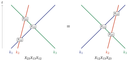
Theorem 13.3 (Three-body consistency). Let the two-body problem give a relation of the form (13.5) with $X=PY$ invertible and unitary, $X_{21}(-u)X_{12}(u)=\Id$ — which for $X$ commuting with $P$ , as Yang’s do, is $X(u)X(-u)=\Id$ . The contact conditions on the three-body ansatz (13.4) have a solution for every incoming amplitude $A_{\mathrm{id}}$ if and only if $X_{12}(u_{12})\,X_{13}(u_{13})\,X_{23}(u_{23}) =X_{23}(u_{23})\,X_{13}(u_{13})\,X_{12}(u_{12}) .$ (13.6) The outgoing amplitude is then $B_{w_0}=X_{12}X_{13}X_{23}\,B_{\mathrm{id}}$ .

Proof. The six amplitudes sit at the vertices of a hexagon, the permutations of $S_3$ , and the conditions sit on its six edges, each an invertible map from one vertex to the next (Lemma 13.2); unitarity says that the map read from the other end is its inverse, so each edge carries one relation. Given $B_{\mathrm{id}}$ , going round either side fixes everything up to $B_{w_0}$ ; the two values agree for every $B_{\mathrm{id}}$ if and only if the two products of Figure 13.1 are equal, which is (13.6). If they are equal, the amplitudes so defined satisfy every edge, and $A_\sigma=\Pi_\sigma^{-1}B_\sigma$ .

This is “derived, not postulated”: nothing was assumed but that the three-body wave is a sum of rearranged plane waves, and the equation is what that costs. The logic runs one way: the equation is necessary for a consistent factorised ansatz; it does not by itself prove that an interaction is non-diffractive.

Proposition 13.4 (Yang’s matrix satisfies it). $X_{\mathrm B}$ and $X_{\mathrm F}$ of (13.3) satisfy (13.6) for all real $k_1,k_2,k_3$ , for every $d$ .

Proof. The scalar factors $1/(u_{ab}+\ii)$ are the same three on both sides. For $X_{\mathrm B}$ what is left is (13.6) for $\Rmat(u)=u-\ii P$ . Expand both sides; the transpositions obey $P_{12}P_{13}=P_{13}P_{23}=P_{23}P_{12}=:C$ and $P_{13}P_{12}=P_{12}P_{23}=P_{23}P_{13}=C^{-1}$ , and $P_{12}P_{13}P_{23}=P_{13}=P_{23}P_{13}P_{12}$ . The terms with no $P$ , one $P$ and three $P$ ’s agree term by term. The terms with two are $-(u_{23}+u_{12})C-u_{13}C^{-1}$ on the left and $-u_{13}C-(u_{12}+u_{23})C^{-1}$ on the right, and they agree because $u_{13}=u_{12}+u_{23} :$ the spectral parameters are differences of momenta, so they add. For $X_{\mathrm F}$ , replace every $u$ by $-u$ .

The proof used only the form $u-\ii P$ and the additivity of $u$ ; the variant $u-\ii(1+\epsilon u)P$ , just as harmless-looking, fails (13.6) for every $\epsilon\ne0$ (the check script; the reading at the end).

Scalar $S$ : automatic. Without labels, $d=1$ , $P=1$ and $X=(u-\ii)/(u+\ii)=S$ : both sides are $S_{12}S_{13}S_{23}$ , and the order of the crossings does not matter. The Toda chain is in the same position: no labels, numbers (displacements) at the crossings, and its braid relation (Figure 12.6) is the scalar, automatic case. The equation earns its keep only with labels.

$N$ particles sketched. The amplitudes sit on the permutations of $S_N$ , the conditions on the edges $\sigma\to\sigma s_j$ , and they are consistent if every closed walk multiplies to $\Id$ . By Coxeter’s presentation of $S_N$ (cited from Gaudin §10.1) the closed walks are generated by an edge and back (unitarity, $X_{21}(-u)X_{12}(u)=\Id$ ), the squares $s_js_l=s_ls_j$ , $\abs{j-l}\ge2$ (automatic: four different lines), and the hexagons $s_js_{j+1}s_j=s_{j+1}s_js_{j+1}$ (the Yang–Baxter equation). So the Yang–Baxter equation and unitarity make the $N$ -body factorised ansatz consistent; the check script confirms it for $N=4$ .

13.4 Factorised scattering

The $N$ -body S-matrix is the ordered product of two-body matrices, one per pair of momentum lines, in the order the lines cross, $S_N=\prod_{\text{crossings, in time order}}X_{ab}(u_{ab}),$ (13.7) and by the Yang–Baxter equation every order of crossings gives the same product: the many-body problem is determined by the two-body one. On a ring, carrying one particle round gives, as in Theorem 11.3, a condition — now on a vector of labels: an eigenvalue problem for a product of $X$ ’s, a transfer matrix, solved by the nested algebraic Bethe ansatz (optional lecture C).

13.5 What it buys

The consistency condition of Part II, derived rather than postulated: a factorised three-body wave exists for every incoming amplitude exactly when the two orders of Figure 13.1 agree.
Yang’s matrix, $\Rmat(u)=u-\ii P$ up to a scalar, the R-matrix from which Lecture 14 builds the Heisenberg chain’s commuting transfer matrices.
Factorised scattering for $N$ particles, sketched: with unitarity, the equation makes every order of crossings give the same product (13.7).

13.6 Caveats, in one place

Status. Proposition 13.1, Theorem 13.3 and Proposition 13.4 are proved. The $N$ -body statement is sketched, with Coxeter’s presentation of $S_N$ cited, and checked for $N=4$ . The Zamolodchikov–Faddeev algebra of the reading is cited.
Necessary, not sufficient. The equation is what a consistent factorised ansatz costs. It does not by itself prove that an interaction is non-diffractive.
Unitarity is a second condition, $X(u)X(-u)=\Id$ for matrices that commute with $P$ ; Yang’s satisfy it.
Without labels the equation is automatic, so Lecture 11’s gas and Lecture 12’s chain never tested it.

13.7 Three lines crossing, and the equation written down

Suppose three-body scattering is a sequence of two-body events. There are two ways for three lines to cross pairwise. Draw each particle’s path in space and time (a world line), with time running up. Three world lines with three different speeds meet pairwise in three crossings, and the middle line can pass either below or above the crossing of the other two (Figure 13.2). The two orders are different sequences of two-body events, and they describe the same three-body collision. They must agree.

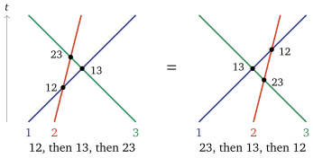
Figure 13.2. The picture behind the Yang–Baxter equation. Three particles, the same three speeds in both panels, time running up; only the starting offsets differ. The middle world line passes on one side of the crossing of the other two or on the other, so the three two-body events (dots, labelled by the pair) happen in opposite orders. If three-body scattering is nothing but its two-body events, both orders must give the same result. Figure 12.6 is its classical form for the Toda chain, and Figure 13.1 its quantum form.

This requirement is the Yang–Baxter equation, and it is a condition on the two-body scattering alone. For particles with nothing but a momentum it is automatic: each two-body event then contributes a number (classically, a shift in position; quantum mechanically, a phase), and numbers do not care about order. It bites when the particles carry an internal label — a spin, a colour — that a two-body event can exchange. Then each event is a matrix, matrices do not commute, and the equation is a strong constraint: a system whose two-body scattering fails it cannot scatter factorisably. Yang met it in 1967 as the consistency condition for exactly this kind of many-body scattering; Baxter met it in 1972 in the statistical mechanics of two-dimensional lattices.

The equation does not organise everything. The geometry of Part I — phase space, the Liouville–Arnold theorem, action-angle variables, the failure of integrability — owes it nothing. Nor does all of the algebra: the Lax pairs of Lecture 8 and the reduction behind Calogero–Moser (optional lecture B) do not come from it. What rests on it is one construction: commuting transfer matrices built from an $\rmat$ -matrix. There the classical equation is the model-independent condition that makes the bracket consistent — sufficient, not forced, as Lecture 14’s reading explains — and it is realised by the periodic chain of Lecture 9; the quantum equation plays the same part from Lecture 14 on. (The open chain of Lecture 9’s readings has an $\rmat$ -matrix bracket too, but of another kind, and its involution does not need the equation.) That construction is the course’s spine from Part I into Part II.

For readers who have met spin: let two particles each carry a spin- $\frac12$ , and let them be fermions with a contact interaction. Their two-body scattering acts on the four-dimensional space $\C^{2}\otimes\C^{2}$ of the pair by $X_{\mathrm F}(u)=-L(u)/(u+\ii)$ of (13.3), with numerator $L(u)=u\,\Id+\ii\,\perm,$ where $\perm$ swaps the two spins and $u$ is the difference of the two particles’ rapidities, a parametrisation of their momenta. The scalar $-1/(u+\ii)$ makes $X_{\mathrm F}$ unitary, and it is the same three factors on both sides of the equation below, so the equation can be written with $L$ . For three particles, write $L_{12}(u)$ for $L(u)$ acting on the spins of particles $1$ and $2$ and as the identity on the third, and so on. The two orders of Figure 13.2 are the two sides of $L_{12}(u-v)\,L_{13}(u)\,L_{23}(v) =L_{23}(v)\,L_{13}(u)\,L_{12}(u-v),$ an identity between $8\times8$ matrices. For this $L$ it holds for all $u$ and $v$ ; for the apparently harmless variant $u\,\Id+\ii(1+cu)\perm$ it fails for every $c\ne0$ (scripts/check-l0-algebra.py, group 6). This is Yang’s solution (1967), the one behind the Heisenberg chain of Lecture 10. This lecture derives the equation from three-body consistency, and Lecture 14 builds the rest of Part II on it.

13.8 The two coordinate Bethe ansätze, side by side

**Table 13.1.** The two coordinate Bethe ansätze side by side.
	Heisenberg chain (Lecture 10)	delta gas (Lecture 11)
particles	magnons on a lattice	bosons on a line
variable	rapidity $\lambda$ , $e^{\ii k}=(\lambda+\ii/2)/(\lambda-\ii/2)$	momentum $k$
two-body $S$	$(\lambda-\ii)/(\lambda+\ii)$	$(k-\ii c)/(k+\ii c)$ , the same at $k=c\lambda$
Bethe equations	$e^{\ii k_jN}\prod_{l\ne j}S(\lambda_j-\lambda_l)=1$	$e^{\ii k_jL}\prod_{l\ne j}S(k_j-k_l)=1$
energy	$-\sum2J/(4\lambda_j^{2}+1)$	$\sum k_j^{2}$
complex roots	strings: bound states	none for $c>0$
eigenfunction	sketched	proved
completeness	numerics; a reformulation (cited)	proved (cited)

13.9 The Zamolodchikov–Faddeev algebra

Factorised scattering has an algebraic shorthand. Give each asymptotic particle an operator $Z(k)$ that creates it, with one component per label, and write $Z_a(k)$ for $Z(k)$ with its label in tensor slot $a$ (Lecture 9’s leg notation). Postulate the exchange relation $Z_1(k_1)\,Z_2(k_2)=X_{12}(u_{12})\,Z_2(k_2)\,Z_1(k_1):$ reordering two neighbours costs one two-body matrix. A product of three can be reversed in two ways, giving $X_{12}X_{13}X_{23}\,Z_3Z_2Z_1$ and $X_{23}X_{13}X_{12}\,Z_3Z_2Z_1$ : the two sides of (13.6). Exchanging twice returns the product to itself only if $X(u)X(-u)=\Id$ (for matrices that commute with $P$ , as Yang’s do): unitarity. This is the Zamolodchikov–Faddeev algebra (Zamolodchikov and Zamolodchikov 1979; Faddeev 1980) cited. In relativistic field theory, where it was born, the two-body matrix obeys a third condition, crossing symmetry, which relates a particle going forward in time to an antiparticle going backwards. It has no counterpart for the non-relativistic particles of this course, which is one reason field theory is outside it (Lecture 0).

Summary

Labels (Proposition 13.1): two labelled particles scatter with Yang’s matrix $Y$ ; along the momentum lines $X=PY$ , which for bosons is $\Rmat(u)/(u+\ii)$ with $\Rmat(u)=u-\ii P$ and $u=(k_1-k_2)/c$ .
Three-body consistency (Theorem 13.3): given unitarity, the factorised ansatz has a solution for every incoming amplitude if and only if $X_{12}X_{13}X_{23}=X_{23}X_{13}X_{12}$ , the Yang–Baxter equation.
Yang’s matrix satisfies it (Proposition 13.4), because the spectral parameters are differences of momenta and add; a harmless-looking variant fails.
$N$ particles (sketched): unitarity and the equation make the ansatz consistent, and the $N$ -body S-matrix is an ordered product of two-body matrices (13.7).
Next: Lecture 14 meets the same equation as the RLL relation, and builds commuting transfer matrices from it.

Worked in the tutorial: Exercise Sheet 13.

References

C. N. Yang, Phys. Rev. Lett. 19 (1967) 1312 (labelled particles, and the equation); M. Gaudin, The Bethe Wavefunction, trans. J.-S. Caux, Cambridge University Press (2014), §10.1 (Coxeter’s presentation and the $N$ -body ansatz); B. Sutherland, Beautiful Models, World Scientific (2004), Chapter 2 (non-diffraction); R. J. Baxter, Exactly Solved Models in Statistical Mechanics, Academic Press (1982) (the equation on lattices); A. B. Zamolodchikov and Al. B. Zamolodchikov, Ann. Phys. 120 (1979) 253; L. D. Faddeev, Sov. Sci. Rev. C1 (1980) 107 (the exchange algebra).

The whole bibliography, lecture by lecture →