15.1 The question

Lecture 10 found the Heisenberg chain’s eigenstates by guessing a wavefunction, and Lecture 14 showed that its transfer matrices commute. So the question is

how do you diagonalise the transfer matrix without writing a wavefunction?

The answer: the Hamiltonian is in the family (Proposition 15.3); vectors built from one reference state by a creation operator $B$ are eigenvectors when the Bethe equations hold (Theorem 15.7 and Corollary 15.9), and the eigenvalue gives the energy and momentum (Proposition 15.10). The worked example is one magnon (15.5).

15.2 The regular point: the shift and the Hamiltonian

At $\lambda=0$ the transfer matrix is the shift

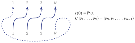
At $\lambda=0$ the Lax operator is a pure swap, $\Lop{an}(0)=\ii P_{an}$ , and every vertex of the loop turns (Figure 15.1). The state that enters the loop is deposited on site $1$ , while site $1$ ’s old state is carried along the auxiliary line to site $2$ ; the loop passes each site’s state on to the next, and the trace brings the last one round to site $1$ .

Figure 15.1. The regular point. At

\lambda=0

every vertex is a swap: the state arriving from below on site

n

turns onto the auxiliary line and leaves upward on site

n+1

. The dashed arc is the trace, which carries site

N

’s state round to site

1

. The loop has become the cyclic shift.

Proposition 15.1 (The shift). $\transfer(0)=\ii^{N}U$ , where $U$ is the cyclic shift, $U(v_1\otimes v_2\otimes\cdots\otimes v_N)=v_N\otimes v_1\otimes\cdots\otimes v_{N-1}$ : the state of site $n$ moves to site $n+1$ . Explicitly $U=P_{N,N-1}P_{N,N-2}\cdots P_{N,1}$ . On a magnon of momentum $k$ (10.5), $U=e^{-\ii k}$ .

Proof. $\mono_a(0)=\ii^{N}P_{aN}P_{a,N-1}\cdots P_{a1}$ . The identity $P_{aN}P_{am}=P_{Nm}P_{aN}$ (the first equality chain of (14.3), relabelled) moves $P_{aN}$ to the right end one factor at a time: $P_{aN}\cdots P_{a1}=P_{N,N-1}\cdots P_{N,1}\,P_{aN}$ . Now $\tra P_{aN}=\Id$ , since $P=\sum_{ij}E_{ij}\otimes E_{ji}$ and $\tr E_{ij}=\delta_{ij}$ . Applying $P_{N,1}$ , then $P_{N,2}$ , …, to $v_1\otimes\cdots\otimes v_N$ puts $v_N$ on site $1$ , $v_1$ on site $2$ , and so on. On $\ket x$ , a down spin at $x$ , $U\ket x=\ket{x+1}$ , so $U\sum_xe^{\ii kx}\ket x=e^{-\ii k}\sum_xe^{\ii kx}\ket x$ .

So the first member of the family is the lattice translation, and the total momentum $K$ is read off from $U=e^{-\ii K}$ . Since $\transfer(0)$ is invertible, the operator $\transfer(0)^{-1}\transfer(\lambda)=\Id+O(\lambda)$ has a logarithm near $\lambda=0$ , a power series in $\lambda$ whose coefficients commute with every $\transfer(\mu)$ . Write $\frac{\dd^{k}}{\dd\lambda^{k}}\ln\transfer(\lambda)\big|_0$ for $k!$ times its $\lambda^{k}$ coefficient; for $k=1$ it is $\transfer(0)^{-1}\transfer'(0)$ .

The Hamiltonian

Lemma 15.2 (One vertex straightened). Delete the factor $P_{am}$ from $P_{aN}\cdots P_{a1}$ and trace over $a$ . The result is $U\,P_{m-1,m}$ , with $P_{0,1}:=P_{N,1}$ closing the ring.

Proof (★). Let $F=P_{aN}\cdots P_{a1}$ and let $F_m$ be $F$ without $P_{am}$ . For $m\ge2$ , $P_{am}P_{a,m-1}=P_{a,m-1}P_{m-1,m}$ (both are the same $3$ -cycle, (14.3)), and $P_{m-1,m}$ commutes with every $P_{ak}$ , $k<m-1$ . So $F=F_m\,P_{m-1,m}$ , hence $F_m=F\,P_{m-1,m}$ and $\tra F_m=U\,P_{m-1,m}$ . For $m=1$ , $F_1$ is the product for the sites $2,\dots,N$ alone, whose trace is the cyclic shift of those sites, and that is $UP_{N,1}$ .

Proposition 15.3 (The Hamiltonian from the transfer matrix). $\frac{\dd}{\dd\lambda}\ln\transfer(\lambda)\Big|_{0} =\transfer(0)^{-1}\transfer'(0)=-\ii\sum_{n=1}^{N}P_{n,n+1}, \qquad\text{so}\qquad H=\frac J2\Big(\ii\,\frac{\dd}{\dd\lambda}\ln\transfer(\lambda)\Big|_{0}-N\Big)$ (15.1) is the Heisenberg Hamiltonian (10.2), and it commutes with $\transfer(\mu)$ for every $\mu$ .

Proof. $\Lop{an}'=\Id$ , so by Leibniz $\transfer'(0)$ is the sum over $m$ of the product with the $m$ -th factor replaced by $\Id$ : $\transfer'(0)=\ii^{N-1}\sum_m\tra F_m=\ii^{N-1}U\sum_mP_{m-1,m}$ by Lemma 15.2. Multiply by $\transfer(0)^{-1}=\ii^{-N}U^{-1}$ . Then use $H=\tfrac J2\sum(P_{n,n+1}-1)$ .

So the Hamiltonian sits in the commuting family, and every $\transfer(\mu)$ is conserved.

15.3 The monodromy matrix and its reference state

Lecture 14 built, for the Heisenberg chain of $N$ sites, the Lax operator $\Lop{an}(\lambda)=\lambda+\ii P_{an}$ (14.2), the monodromy matrix and the transfer matrix $\mono_a(\lambda)=\Lop{aN}(\lambda)\cdots\Lop{a1}(\lambda) =\begin{pmatrix}A(\lambda)&B(\lambda)\\ C(\lambda)&D(\lambda)\end{pmatrix}_{\!a}, \qquad \transfer(\lambda)=A(\lambda)+D(\lambda),$ (15.2) and proved the $RTT$ relation (14.6), $\Rmat_{ab}(\lambda-\mu)\mono_b(\mu)\mono_a(\lambda)=\mono_a(\lambda)\mono_b(\mu)\Rmat_{ab}(\lambda-\mu)$ with $\Rmat(\lambda)=\lambda-\ii P$ , and $\comm{\transfer(\lambda)}{\transfer(\mu)}=0$ (Theorem 14.3). The Hamiltonian is $H=\frac J2\big(\ii\frac{\dd}{\dd\lambda}\ln\transfer|_0-N\big)$ and the shift is $\transfer(0)=\ii^{N}U$ (Proposition 15.3, Proposition 15.1). The goal is now the spectrum of $\transfer(\lambda)$ : one family of eigenvectors, good for every $\lambda$ at once, and with it the spectrum of $H$ .

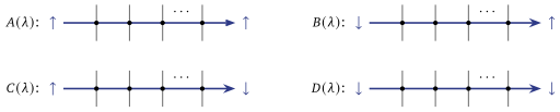
The entries $A,B,C,D$ are operators on the chain, and Figure 15.2 says what each does. Read the auxiliary line as carrying a spin from left to right: it enters in the state of the column index and leaves in the state of the row index. At every vertex $\Lop{an}=\lambda+\ii P_{an}$ either lets both spins pass or swaps them, so the number of down spins on the auxiliary line and the chain together is conserved: $P$ commutes with $S^{z}$ of the pair it acts on. Hence $A$ and $D$ conserve $S^{z}$ of the chain, $B$ (in $\downarrow$ , out $\uparrow$ ) leaves one more down spin on the chain than it found, and $C$ takes one away: $\comm{S^{z}}{B(\lambda)}=-B(\lambda),\qquad \comm{S^{z}}{C(\lambda)}=C(\lambda),\qquad \comm{S^{z}}{A(\lambda)}=\comm{S^{z}}{D(\lambda)}=0 .$ (15.3)

Figure 15.2. The four entries of the monodromy matrix: the row of Figure 14.2 with its two ends fixed, the column index entering on the left (site

1

first) and the row index leaving on the right.

The obvious state to start from is the ferromagnetic one, all spins up, $\ket0=\ket{\uparrow\uparrow\cdots\uparrow}$ , the $\ket\Uparrow$ of Lecture 10. On it every Lax operator is triangular.

Proposition 15.4 (The reference state). For all $\lambda$ , $A(\lambda)\ket0=(\lambda+\ii)^{N}\ket0,\qquad D(\lambda)\ket0=\lambda^{N}\ket0, \qquad C(\lambda)\ket0=0,$ (15.4) and, with $\ket n$ the state with one down spin at site $n$ , $B(v)\ket0=\ii\sum_{n=1}^{N}v^{\,n-1}(v+\ii)^{N-n}\ket n =\ii\,\frac{(v+\ii)^{N}}{v}\sum_{n=1}^{N}\Big(\frac{v}{v+\ii}\Big)^{n}\ket n \quad(v\ne0,-\ii).$ (15.5)

Proof. From (14.2), acting on site $n$ in the state $\uparrow$ , $\Lop{an}(\lambda)\ket{\uparrow}_n=\begin{pmatrix}(\lambda+\ii)\ket\uparrow_n&\ii\ket\downarrow_n\\ 0&\lambda\ket\uparrow_n\end{pmatrix}_{\!a},$ since $S^{+}\ket\uparrow=0$ , $S^{-}\ket\uparrow=\ket\downarrow$ and $S^{z}\ket\uparrow=\tfrac12\ket\uparrow$ . Sites $1,\dots,N$ are acted on by different factors of (15.2), so on $\ket0$ the monodromy is a product of triangular $2\times2$ matrices. Its lower-left entry vanishes and its diagonal entries are the products of the diagonals. The upper-right entry is a sum over the one place where the product steps from the second row to the first: on sites $1,\dots,n-1$ the factor is $\lambda$ , at site $n$ it is $\ii\ket\downarrow_n$ , and on sites $n+1,\dots,N$ it is $\lambda+\ii$ . Set $\lambda=v$ .

So $B$ creates. For $v\ne0,-\ii$ , $B(v)\ket0$ is a plane wave: its amplitude on site $n$ is proportional to $e^{\ii kn}$ with $e^{\ii k}=\frac{v}{v+\ii},\qquad\text{i.e., in the rapidity of \text{(10.6)},}\qquad v=-\lambda-\frac\ii2 .$ (15.6) It is the magnon $\ket k$ of (10.5) for every such $v$ , not only for the $N$ values allowed on the ring; periodicity has not been imposed, and $B(v)\ket0$ is an eigenvector of $H$ only when $e^{\ii kN}=1$ . At the two excluded values the vector is not a plane wave at all but a single site, $B(0)\ket0=\ii^{N}\ket1$ and $B(-\ii)\ket0=\ii(-\ii)^{N-1}\ket N$ ; they are the ends $k\to\pm\ii\infty$ of (15.6), and they return in §15.5 as the singular pair. The arguments $v$ of the creation operators play the part of rapidities, shifted and reflected.

15.4 The exchange relations

To act with $\transfer=A+D$ on a product of $B$ ’s, one needs to move $A$ and $D$ to the right, past each $B$ , until they reach $\ket0$ . The $RTT$ relation is sixteen such rules, one for each entry of a $4\times4$ matrix in the auxiliary spaces $a\otimes b$ .

Lemma 15.5 ( $RTT$ , entry by entry). Write $T_{11}=A$ , $T_{12}=B$ , $T_{21}=C$ , $T_{22}=D$ . For all $i,j,k,l\in\{1,2\}$ , $(\lambda-\mu)\,T_{jl}(\mu)T_{ik}(\lambda)-\ii\,T_{il}(\mu)T_{jk}(\lambda) =(\lambda-\mu)\,T_{ik}(\lambda)T_{jl}(\mu)-\ii\,T_{il}(\lambda)T_{jk}(\mu).$ (15.7)

Proof (★). In the leg notation of Definition 9.2, the $(ij),(kl)$ entry of $\mono_a(\lambda)\mono_b(\mu)$ is $T_{ik}(\lambda)T_{jl}(\mu)$ , and of $\mono_b(\mu)\mono_a(\lambda)$ it is $T_{jl}(\mu)T_{ik}(\lambda)$ : the same operators in the other order, which now matters. Multiplying on the right by $P_{ab}$ exchanges the column indices $k$ and $l$ , and conjugating by $P_{ab}$ exchanges the legs, so $P\,\mono_b(\mu)\mono_a(\lambda)=\mono_a(\mu)\mono_b(\lambda)\,P$ . With $\Rmat=(\lambda-\mu)-\ii P$ , (14.6) reads $(\lambda-\mu)\,\mono_b(\mu)\mono_a(\lambda)-\ii\,\mono_a(\mu)\mono_b(\lambda)P =(\lambda-\mu)\,\mono_a(\lambda)\mono_b(\mu)-\ii\,\mono_a(\lambda)\mono_b(\mu)P,$ whose $(ij),(kl)$ entry is (15.7).

Three of the sixteen are needed. Write $f(u)=\frac{u-\ii}{u},\qquad g(u)=\frac{\ii}{u}.$ (15.8)

Proposition 15.6 (The exchange relations). For all $\lambda,\mu$ , and for $\lambda\ne\mu$ in the last two, $B(\lambda)B(\mu)=B(\mu)B(\lambda),$ (15.9) $A(\lambda)B(\mu)=f(\lambda-\mu)\,B(\mu)A(\lambda)+g(\lambda-\mu)\,B(\lambda)A(\mu),$ (15.10) $D(\lambda)B(\mu)=f(\mu-\lambda)\,B(\mu)D(\lambda)-g(\lambda-\mu)\,B(\lambda)D(\mu).$ (15.11)

Proof. Each is one entry of (15.7). With $(i,j,k,l)=(1,1,2,2)$ both products on each side are $B$ ’s: $(\lambda-\mu-\ii)B(\mu)B(\lambda)=(\lambda-\mu-\ii)B(\lambda)B(\mu)$ , which gives (15.9) for $\lambda-\mu\ne\ii$ , and for all $\lambda,\mu$ because both sides are polynomials. With $(1,1,1,2)$ , $(\lambda-\mu-\ii)B(\mu)A(\lambda)=(\lambda-\mu)A(\lambda)B(\mu)-\ii B(\lambda)A(\mu)$ ; divide by $\lambda-\mu$ . With $(1,2,2,2)$ , $(\lambda-\mu)D(\mu)B(\lambda)-\ii B(\mu)D(\lambda)=(\lambda-\mu-\ii)B(\lambda)D(\mu)$ ; exchange the names $\lambda\leftrightarrow\mu$ and divide by $\lambda-\mu$ .

Read (15.10) as a rule for moving $A(\lambda)$ one step to the right. Either $A$ keeps its argument, and pays $f(\lambda-\mu)$ , or $A$ and $B$ exchange arguments, at the price $g(\lambda-\mu)$ : the two terms of $\Rmat=(\lambda-\mu)-\ii P$ , straight through or swapped.

15.5 Bethe vectors: wanted and unwanted terms

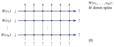
For complex numbers $v_1,\dots,v_M$ define the Bethe vector $\Psi(v_1,\dots,v_M)=B(v_1)B(v_2)\cdots B(v_M)\ket0 .$ (15.12) By (15.9) it is symmetric in the $v_j$ , and by (15.3) it has $S^{z}=\tfrac N2-M$ : $M$ down spins, each brought in by one auxiliary line (Figure 15.3). Beyond one magnon (15.5), no wavefunction will be written.

Figure 15.3. A Bethe vector. The reference state (bottom) is all up; each creation operator is a row that enters with a down spin and leaves with an up spin, so it deposits one down spin on the chain, spread over the sites with amplitudes set by its argument. Operators act from the bottom up:

B(v_M)

first.

Theorem 15.7 (Wanted and unwanted terms). Let $v_1,\dots,v_M$ be pairwise distinct and $\lambda\notin\{v_1,\dots,v_M\}$ . Then $\transfer(\lambda)\,\Psi(v_1,\dots,v_M) =\Lambda(\lambda)\,\Psi(v_1,\dots,v_M) +\sum_{j=1}^{M}\mathcal M_j(\lambda)\,B(\lambda)\prod_{k\ne j}B(v_k)\ket0,$ (15.13) with $\Lambda(\lambda)=(\lambda+\ii)^{N}\prod_{j=1}^{M}\frac{\lambda-v_j-\ii}{\lambda-v_j} +\lambda^{N}\prod_{j=1}^{M}\frac{\lambda-v_j+\ii}{\lambda-v_j},$ (15.14) $\mathcal M_j(\lambda)=\frac{\ii}{\lambda-v_j}\Big[(v_j+\ii)^{N}\prod_{k\ne j}\frac{v_j-v_k-\ii}{v_j-v_k} -v_j^{N}\prod_{k\ne j}\frac{v_j-v_k+\ii}{v_j-v_k}\Big].$ (15.15)

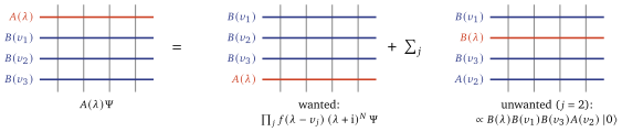
The first term of (15.13) is wanted: it is a multiple of $\Psi$ . The others are unwanted: in each, one creation operator has had its argument replaced by $\lambda$ (Figure 15.4).

Figure 15.4. Moving

A(\lambda)

down through the creation rows (here

M=3

; rows act from the bottom up, as in Figure 15.3). If

A

keeps its argument at every exchange it reaches

\ket0

A(\lambda)

and returns

(\lambda+\ii)^{N}

: the wanted term. If it exchanges arguments with

B(v_j)

it reaches

\ket0

A(v_j)

, returning

(v_j+\ii)^{N}

, and the

j

-th creation row now carries

\lambda

: an unwanted term. The argument

\lambda

(red) is never lost, only handed on.

D(\lambda)

does the same with

\lambda^{N}

and

v_j^{N}

Where do the two kinds of term come from? Each use of (15.10) replaces $A(x)B(y)$ by terms $B(y)A(x)$ and $B(x)A(y)$ : the set of arguments $\{x,y\}$ is preserved. Moving $A(\lambda)$ to the right through $B(v_1)\cdots B(v_M)$ , every term therefore ends as $M$ creation operators and one $A$ , whose arguments together are $\lambda,v_1,\dots,v_M$ . Either $A$ ends with $\lambda$ , and the $B$ ’s make $\Psi$ ; or it ends with some $v_j$ , and the $B$ ’s make $B(\lambda)\prod_{k\ne j}B(v_k)$ . The coefficients are easy to guess. The wanted one comes from keeping the argument at every step: $\prod_kf(\lambda-v_k)$ . For the $j$ -th unwanted one, use (15.9) to put $B(v_j)$ first: $A$ must exchange at the first step, paying $g(\lambda-v_j)$ and becoming $A(v_j)$ , and then keep $v_j$ at every later step, paying $f(v_j-v_k)$ .

Lemma 15.8 (Moving $A$ and $D$ through the creation operators). For pairwise distinct $v_1,\dots,v_M$ and $\lambda\notin\{v_k\}$ , $\begin{split} A(\lambda)\prod_{k=1}^{M}B(v_k)={}&\prod_{k}f(\lambda-v_k)\prod_{k}B(v_k)\,A(\lambda)\\ &+\sum_{j=1}^{M}g(\lambda-v_j)\prod_{k\ne j}f(v_j-v_k)\,B(\lambda)\prod_{k\ne j}B(v_k)\,A(v_j), \end{split}$ (15.16) and the same for $D$ with $f(u)\to f(-u)$ and $g(u)\to-g(u)$ throughout.

Proof (★). The guess put $B(v_j)$ first, a different order for each $j$ , so it does not yet show that one expansion has all these coefficients at once. Induct on $M$ ; $M=1$ is (15.10). For $M\ge2$ apply (15.10) to $A(\lambda)B(v_1)$ , then the hypothesis for $M-1$ to both $A(\lambda)$ and $A(v_1)$ acting on $B(v_2)\cdots B(v_M)$ . The wanted term and the term ending in $A(v_1)$ come out as claimed. A term ending in $A(v_j)$ , $j\ge2$ , arrives twice, with total coefficient $\prod_{k\ne 1,j}f(v_j-v_k)$ times $f(a)g(b)+g(a)g(b-a)$ , where $a=\lambda-v_1$ , $b=\lambda-v_j$ ; a line of algebra gives $f(a)g(b)+g(a)g(b-a)=g(b)f(a-b)$ , and $f(a-b)=f(v_j-v_1)$ is the missing factor. For $D$ the same identity holds for $f(-u)$ and $-g(u)$ , being the one above at $(-a,-b)$ . (The check script confirms (15.16) as an operator identity for two and three sites.)

Proof of Theorem 15.7. Apply Lemma 15.8 to $\ket0$ and use (15.4): $A(\lambda)\ket0=(\lambda+\ii)^{N}\ket0$ , $A(v_j)\ket0=(v_j+\ii)^{N}\ket0$ , $D(\lambda)\ket0=\lambda^{N}\ket0$ , $D(v_j)\ket0=v_j^{N}\ket0$ . Since $f(\lambda-v)=(\lambda-v-\ii)/(\lambda-v)$ and $f(v-\lambda)=(\lambda-v+\ii)/(\lambda-v)$ , the wanted terms of $A$ and $D$ add to (15.14), and the unwanted coefficients to (15.15).

Corollary 15.9 (The algebraic Bethe ansatz). Call the roots regular if they are pairwise distinct and none is $0$ or $-\ii$ . For pairwise distinct $v_1,\dots,v_M$ , all the unwanted coefficients vanish if and only if $(v_j+\ii)^{N}\prod_{k\ne j}(v_j-v_k-\ii)=v_j^{N}\prod_{k\ne j}(v_j-v_k+\ii), \qquad j=1,\dots,M.$ (15.17) If they hold, $\Psi(v_1,\dots,v_M)$ is either zero or a simultaneous eigenvector of every $\transfer(\lambda)$ , with eigenvalue $\Lambda(\lambda)$ , which is then a polynomial. Under $v_j=-\lambda_j-\tfrac\ii2$ (15.6), and when no factor in (10.15) vanishes or diverges, (15.17) is the system (10.15) of Lecture 10.

Proof. $\mathcal M_j$ is $\ii/(\lambda-v_j)$ times the difference of the two sides of (15.17), divided by $\prod_{k\ne j}(v_j-v_k)\ne0$ . If (15.17) holds, (15.13) says $\transfer(\lambda)\Psi=\Lambda(\lambda)\Psi$ for $\lambda\notin\{v_j\}$ . If $\Psi\ne0$ , pick a component $\Psi_x\ne0$ : then $\Lambda(\lambda)=(\transfer(\lambda)\Psi)_x/\Psi_x$ is a polynomial in $\lambda$ , and the eigenvalue equation extends to every $\lambda$ . For the last statement substitute: $v_j+\ii=-(\lambda_j-\tfrac\ii2)$ , $v_j=-(\lambda_j+\tfrac\ii2)$ and $v_j-v_k\pm\ii=-(\lambda_j-\lambda_k\mp\ii)$ , so (15.17) becomes $(\lambda_j-\tfrac\ii2)^{N}\prod(\lambda_j-\lambda_k+\ii)=(\lambda_j+\tfrac\ii2)^{N}\prod(\lambda_j-\lambda_k-\ii)$ , a common sign $(-1)^{N+M-1}$ having cancelled; divide.

The Bethe equations of Lecture 10 have come back without a wavefunction.

15.6 The eigenvalue

$\Lambda(\lambda)$ is the eigenvalue of the whole commuting family at once, so the eigenvalues of $H$ and of the shift follow from Proposition 15.3 and Proposition 15.1 without further work.

Proposition 15.10 (Momentum and energy from $\Lambda$ ). Let $v_1,\dots,v_M$ be regular roots solving (15.17), with $\Psi\ne0$ , $N\ge2$ , and $\lambda_j=-v_j-\tfrac\ii2$ with momenta $e^{\ii k_j}=(\lambda_j+\tfrac\ii2)/(\lambda_j-\tfrac\ii2)$ . Then $U\Psi=e^{-\ii K}\Psi,\quad K=\sum_jk_j,\qquad\text{and}\qquad H\Psi=E\Psi,\quad E=-\sum_{j=1}^{M}\frac{2J}{4\lambda_j^{2}+1},$ which is (10.16).

Proof. At $\lambda=0$ the second term of (15.14) vanishes with its derivative (it carries $\lambda^{N}$ , $N\ge2$ , and no pole at $0$ since $v_j\ne0$ ). So $\Lambda(0)=\ii^{N}\prod_j(v_j+\ii)/v_j$ , not zero since $v_j\ne-\ii$ , and $\frac{\dd}{\dd\lambda}\ln\Lambda\Big|_0=\frac N{\ii}+\sum_j\Big(\frac1{v_j}-\frac1{v_j+\ii}\Big) =-\ii N+\sum_j\frac{\ii}{v_j(v_j+\ii)} .$ With $v_j=-\lambda_j-\tfrac\ii2$ , $(v_j+\ii)/v_j=(\lambda_j-\tfrac\ii2)/(\lambda_j+\tfrac\ii2)=e^{-\ii k_j}$ and $v_j(v_j+\ii)=\lambda_j^{2}+\tfrac14$ . Now $\transfer(0)=\ii^{N}U$ gives the first claim, and (15.1) gives $E=\frac J2\big(\ii\frac{\dd}{\dd\lambda}\ln\Lambda|_0-N\big) =-\frac J2\sum_j\frac{1}{\lambda_j^{2}+1/4}$ .

Everything Lecture 10 extracted from the wavefunction — the Bethe equations, the energy, the momentum — has come from the monodromy and one reference state, at the price of Lecture 14’s $RTT$ relation.

The return is more than a second derivation. $\Lambda$ fixes the eigenvalue of every conserved charge at once — that of $\frac{\dd^{k}}{\dd\lambda^{k}}\ln\transfer|_0$ is $\frac{\dd^{k}}{\dd\lambda^{k}}\ln\Lambda|_0$ — and the method runs for any model with this $\Rmat$ -matrix, or the trigonometric one of §15.11, and a reference state that $C$ annihilates and on which $A$ and $D$ act by numbers. That includes chains whose sites carry different spectral parameters; for a larger auxiliary space there is more than one kind of creation operator and the ansatz has to be nested — both are what optional lecture C needs.

15.7 What it buys

Lecture 10’s Bethe equations, energy and momentum, a second time, from the monodromy and one reference state (Corollary 15.9 and Proposition 15.10), with the Hamiltonian found in the commuting family (Proposition 15.3). Goal G2 is reached.
The eigenvalue $\Lambda(\lambda)$ of the whole family, by a method that needs a monodromy obeying $RTT$ and a reference state that $C$ annihilates and on which $A$ and $D$ act by numbers.

15.8 Caveats, in one place

Status. Proposition 15.1, Proposition 15.3, Theorem 15.7, Corollary 15.9 and Proposition 15.10 are proved; the proofs of Lemma 15.2, Lemma 15.5 and Lemma 15.8 are readings.
The corollary does not say $\Psi\ne0$ . The singular pair of Lecture 10’s reading, $\{v_1,v_2\}=\{0,-\ii\}$ , satisfies (15.17) (both sides vanish), and $B(0)B(-\ii)\ket0=0$ (the check script, $N=4,6,8$ ), although neither factor alone kills $\ket0$ . Lecture 10’s singular eigenstate comes from the regularisation in that lecture, not from the corollary, which is why Proposition 15.10 is stated for regular roots.
No converse, and no completeness. That an eigenvector forces the Bethe equations is not proved here, and completeness remains Lecture 10’s cited question.

15.9 The tower of local charges

Why the logarithm? Each derivative at $0$ straightens one vertex, which after $U^{-1}$ leaves a bond $P_{m-1,m}$ (Lemma 15.2). Two straightened vertices leave two bonds: far apart, a product of two local operators, which is not local; neighbours, one operator on three sites ( $P_{m,m+1}P_{m-1,m}$ , the check script). The square of the first derivative contains the same far-apart products, and the logarithm cancels them; what is left comes from neighbours and from $P^{2}=\Id$ . For $N\ge4$ $\frac{\dd^{2}}{\dd\lambda^{2}}\ln\transfer(\lambda)\Big|_{0} =N+\sum_{n=1}^{N}\comm{P_{n,n+1}}{P_{n+1,n+2}} =N-\frac{\ii}{2}\,Q_3 ,$ (15.18) with $Q_3$ a range- $3$ charge that commutes with $H$ , found here without a commutator computation sketched; verified at $N=6,7,8$ .

In general, $\frac{\dd^{k}}{\dd\lambda^{k}}\ln\transfer|_0$ is a sum over the ring of one density of range $k+1$ , the same density for every $N$ large enough: a local charge, with range growing with $k$ sketched above; proved by Grabowski and Mathieu 1995; the check script verifies range and $N$ -independence for $k\le 3$ at $N=8,9$ ; they commute by Theorem 14.3. It rests on the regular point, where the Lax operator is a permutation, $\transfer(0)$ is invertible and every vertex only passes states along; at a generic $\lambda$ , $\transfer(\lambda)$ couples all $N$ sites at once.

15.10 Baxter’s T–Q relation

Collect the roots into one polynomial, $Q(\lambda)=\prod_{j=1}^{M}(\lambda-v_j).$ (15.19) Then $\prod_j(\lambda-v_j\mp\ii)/(\lambda-v_j)=Q(\lambda\mp\ii)/Q(\lambda)$ , and (15.14) is, multiplied out, $\Lambda(\lambda)\,Q(\lambda)=(\lambda+\ii)^{N}\,Q(\lambda-\ii)+\lambda^{N}\,Q(\lambda+\ii),$ (15.20) Baxter’s T–Q relation. Baxter found it in 1972 for the eight-vertex model, where the reference-state argument of this lecture does not apply as it stands, by constructing $Q$ as an operator commuting with the transfer matrix. It says the same as (15.14), but it turns the Bethe equations into a statement about polynomials.

Proposition 15.11 (The Bethe equations as analyticity). Let $v_1,\dots,v_M$ be pairwise distinct and define $\Lambda$ by (15.20). Then $\Lambda$ is a polynomial if and only if the $v_j$ satisfy (15.17).

Proof. $\Lambda$ is the right side of (15.20) divided by $Q$ , whose zeros are simple. It is a polynomial iff the right side vanishes at every $v_j$ : $(v_j+\ii)^{N}Q(v_j-\ii)+v_j^{N}Q(v_j+\ii)=0$ . Since $Q(v_j\mp\ii)=\mp\ii\prod_{k\ne j}(v_j-v_k\mp\ii)$ , this is (15.17).

The eigenvalue of $\transfer(\lambda)$ on a common eigenvector is a polynomial in $\lambda$ — the argument in the proof of Corollary 15.9. So the Bethe equations are the condition that the ansatz produce an eigenvalue of the right kind: the apparent poles of (15.14) at the roots must cancel. For $M=1$ , $\Lambda Q=(\lambda+\ii)^{N}(\lambda-v-\ii)+\lambda^{N}(\lambda-v+\ii)$ is divisible by $\lambda-v$ iff $(v+\ii)^{N}=v^{N}$ , that is $e^{\ii kN}=1$ by (15.6): the magnon grid of (10.5).

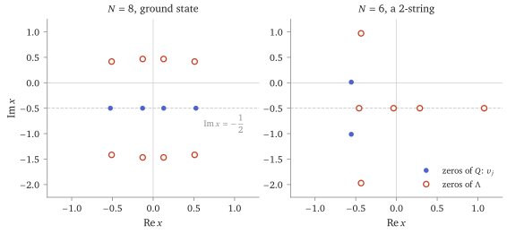
Figure 15.5 shows both polynomials for two states met in Lecture 10. The zeros of $Q$ are the roots; $\Lambda$ , of degree $N$ with leading coefficient $2$ , has its own zeros elsewhere. In Lecture 16 the roots of the ground state fill a line densely and the Bethe equations become an integral equation for their density; Lecture 17’s reading generalises the T–Q relation itself sketched there.

Figure 15.5. The two polynomials of the T–Q relation in the complex plane of their argument

x

. Left: the ground state of

N=8

(

M=4

, real rapidities, so the roots lie on

\operatorname{Im}x=-\tfrac12

); the eight zeros of

\Lambda

lie in two rows, at distance about

1

above and below. Right: the 2-string of

N=6

K=2\pi/3

from Figure 10.5, whose roots

x\approx-\tfrac1{\sqrt3}

and

-\tfrac1{\sqrt3}-\ii

are nearly the singular pair shifted. In both,

\Lambda

is checked to be a polynomial and an eigenvalue of the exact transfer matrix at three complex points. (scripts/figures/tq_roots.py.)

In this form the equations can be asked of any polynomial $Q$ , whether or not it comes from a nonzero Bethe vector. The completeness theorem cited in Lecture 10 (Mukhin, Tarasov and Varchenko) is phrased in this language, for polynomial solutions of (15.20) with extra conditions that absorb the singular solutions.

15.11 The XXZ chain

The anisotropic chain $H_{\mathrm{XXZ}}=J\sum_{n=1}^{N}\Big(S^{x}_nS^{x}_{n+1}+S^{y}_nS^{y}_{n+1} +\XXZ\big(S^{z}_nS^{z}_{n+1}-\tfrac14\big)\Big),\qquad J>0,$ (15.21) is (10.2) at $\XXZ=1$ . Every step of this lecture, and every step of Lecture 14 from the $RLL$ relation onwards, goes through with the linear functions replaced by hyperbolic ones (the $RLL$ relation itself is a separate computation, since Theorem 14.1 was proved inside the group algebra of the permutations of three objects) sketched: the derivation is §§15.3 to 15.6 line by line, with the changes listed in the reading at the end; each formula is checked by the check script. In the basis $\uparrow\uparrow,\uparrow\downarrow,\downarrow\uparrow,\downarrow\downarrow$ the trigonometric R-matrix is $\Rmat(\lambda)=\begin{pmatrix}\sinh(\lambda-\ii\eta)&&&\\ &\sinh\lambda&-\ii\sin\eta&\\ &-\ii\sin\eta&\sinh\lambda&\\ &&&\sinh(\lambda-\ii\eta)\end{pmatrix},\qquad \XXZ=\cos\eta .$ (15.22) It satisfies the Yang–Baxter equation (14.8), and as $\eta\to0$ with $\lambda\to\eta\lambda$ , $\Rmat/\eta\to\lambda-\ii P$ . The Lax operator is again $\Lop{an}(\lambda)=-\Rmat_{an}(-\lambda)$ , as in (14.7), and satisfies $RLL$ in the course’s ordering. On $\ket0$ , $A=\sinh^{N}(\lambda+\ii\eta)$ and $D=\sinh^{N}\lambda$ , and $B(v)\ket0$ is the magnon with $v=-\lambda-\ii\eta/2$ , $e^{\ii k}=\sinh(\lambda+\ii\eta/2)/\sinh(\lambda-\ii\eta/2)$ . The result: $\Lambda(\lambda)=\sinh^{N}(\lambda+\ii\eta)\prod_j\frac{\sinh(\lambda-v_j-\ii\eta)}{\sinh(\lambda-v_j)} +\sinh^{N}\!\lambda\,\prod_j\frac{\sinh(\lambda-v_j+\ii\eta)}{\sinh(\lambda-v_j)},$ (15.23) and the Bethe equations and energy, in $\lambda_j=-v_j-\ii\eta/2$ , $\Big(\frac{\sinh(\lambda_j+\ii\eta/2)}{\sinh(\lambda_j-\ii\eta/2)}\Big)^{N} =\prod_{k\ne j}\frac{\sinh(\lambda_j-\lambda_k+\ii\eta)}{\sinh(\lambda_j-\lambda_k-\ii\eta)}, \qquad E=\sum_j\frac{J\sin^{2}\eta}{\cos\eta-\cosh2\lambda_j}.$ (15.24) At $\XXZ=0$ ( $\eta=\pi/2$ ) the right side is $(-1)^{M-1}$ : the chain is the XX chain, and the equations are the free-fermion grids of Lecture 18.

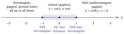
Figure 15.6. The regimes of the XXZ chain (15.21) with

J>0

at zero field. The spectrum is gapless for

-1\le\XXZ\le1

(the shaded interval is the critical regime) and has a gap above the ground states outside it. For

\XXZ<-1

the all-up state is a ground state (the check script,

N=8

); the other labels are cited (Franchini, ch. 4, whose

\XXZ

is minus ours). At

\XXZ=-1

a rotation of every other spin (even

N

) turns the chain into the ferromagnetic Heisenberg chain.

The formulas hold with $\eta$ complex, and the regimes of Figure 15.6 differ in where the roots of the ground state lie; for $\XXZ<-1$ the reference state is a ground state (so is the all-down state). What each regime looks like in the thermodynamic limit is Lecture 16’s business for $\XXZ=1$ and is cited here for the rest cited: Franchini, §§4.3–4.5; Takahashi, ch. 4.

The XXZ chain, step by step

The changes to §§15.3 to 15.6 for the XXZ chain, each checked by the check script:

Regular point. $\transfer(0)=(\ii\sin\eta)^{N}U$ and $H_{\mathrm{XXZ}}=\frac J2\big(\sin\eta\cdot\ii\frac{\dd}{\dd\lambda}\ln\transfer|_0-N\cos\eta\big)$ .
Reference state. $C\ket0=0$ and $B(v)\ket0=\ii\sin\eta\sum_n\sinh^{n-1}\!v\;\sinh^{N-n}(v+\ii\eta)\ket n$ , so for $\sinh v\ne0\ne\sinh(v+\ii\eta)$ the amplitudes are in the ratio $\sinh v/\sinh(v+\ii\eta)=e^{\ii k}$ from site to site (at the excluded values, as in §15.3, the vector sits on one site); one magnon has $E=J(\cos k-\XXZ)$ .
Exchange relations. (15.10) and (15.11) with $f(u)=\sinh(u-\ii\eta)/\sinh u$ and $g(u)=\ii\sin\eta/\sinh u$ ; the identity of Lemma 15.8’s proof holds for these too.

The parametrisation depends on the regime. For $\abs\XXZ<1$ , $\eta$ is real and the rapidities of the ground state are real; for $\XXZ>1$ one writes $\eta=\ii\gamma$ , the hyperbolic functions of $\lambda\pm\ii\eta/2$ become trigonometric after $\lambda\to\ii\lambda$ , and the rapidities live on a circle; for $\XXZ<-1$ the reference state is a ground state. The formulas above hold in all three, with $\eta$ complex (the check script samples $\XXZ=\tfrac12,-\tfrac12,2$ ).

15.12 Norms and scalar products

An eigenvector found by the Bethe ansatz comes unnormalised, and any expectation value needs its norm. For the wavefunction of Lecture 10 with real rapidities, normalised by $A_{\mathrm{id}}=1$ in (10.14), the answer is a determinant: $\sum_{x_1<\dots<x_M}\abs{\psi(x_1,\dots,x_M)}^{2} =\det\Big(\frac{\partial\Phi_j}{\partial k_l}\Big)_{j,l=1}^{M},\qquad \Phi_j=Nk_j+\sum_{l\ne j}\theta_2(\lambda_j-\lambda_l),$ (15.25) the Jacobian of the Bethe equations in the form (10.20), with each $\lambda_l$ a function of $k_l$ cited: Gaudin 1983, proved by Korepin 1982; Korepin, Bogoliubov and Izergin, §§X.1–X.3; the check script verifies it for $N=6,7,8$ , $M\le 4$ . For $M=1$ it says $\sum_x\abs{e^{\ii kx}}^{2}=N$ . In the rapidities, with $F_j$ the left side of the logarithmic equations (10.18), the same determinant is $\det\Big(\frac{\partial\Phi_j}{\partial k_l}\Big) =\prod_{l}\Big(\lambda_l^{2}+\tfrac14\Big)\, \det\Big(\frac{\partial F_j}{\partial\lambda_l}\Big),$ because $\Phi^{\vphantom{1}}_j=N\pi-F_j$ and $\dd k/\dd\lambda=-\theta_1'(\lambda)=-4/(1+4\lambda^{2})$ , and the second matrix is symmetric — the Hessian of a function playing, on the lattice, the part of the convex function of Proposition 11.5. The function whose stationary points are the solutions also measures the size of every Bethe vector.

Real rapidities are a hypothesis, not a convenience. Normalising by $A_{\mathrm{id}}=1$ breaks the symmetry of $\psi$ under relabelling the roots unless $\abs{S(\lambda_j-\lambda_l)}=1$ , while the determinant is symmetric; so no such formula can hold for complex roots in this normalisation. The $2$ -string of Figure 15.5 is a counterexample: there $\sum\abs\psi^{2}=2.16964\ldots$ and the determinant is $176.2159\ldots$ , in the ratio $S(\lambda_1-\lambda_2)=0.0123\ldots$ (the check script). For complex roots the determinant needs the conjugation and ordering factors that the bare formula drops; summing $\abs\psi^{2}$ directly of course still works, and the algebraic scalar product below is the systematic route.

Korepin’s proof does that. The relevant object is the algebraic scalar product $\langle0|\,C(u_1)\cdots C(u_M)\,B(v_1)\cdots B(v_M)\,\ket0 ,$ which the exchange relations for $C$ with $B$ (more entries of (15.7)) reduce to a sum over partitions of the roots (Korepin, Bogoliubov and Izergin, ch. IX). It is a bilinear pairing, not an inner product: in this course’s conventions it equals $(-1)^{M}\norm{\Psi}^{2}$ at coincident real rapidities (the check script), and the sources’ relation $C(\bar\lambda)\propto B(\lambda)^{\dagger}$ belongs to their conventions, not to ours — Lecture 14’s ordering rule once more. The proof itself compares two functions of $M$ free parameters. Let the model be deformed so that the two vacuum eigenvalues $a(\lambda),d(\lambda)$ are arbitrary, and set $z_j=\ii\,\frac{\dd}{\dd\lambda}\ln\frac{a(\lambda)}{d(\lambda)}\Big|_{\lambda_j}, \qquad K_{jl}=\theta_2'(\lambda_j-\lambda_l)=\frac2{1+(\lambda_j-\lambda_l)^{2}} ,$ so that for the chain $z_j=N/(\lambda_j^{2}+\tfrac14)$ and the matrix above is $H_{jl}=\delta_{jl}\big(z_j-\sum_{m\ne j}K_{jm}\big)+(1-\delta_{jl})K_{jl}$ . Both the normalised scalar product — the pairing divided by $\prod_ja(\lambda_j)d(\lambda_j)\prod_{j\ne k}f(\lambda_j-\lambda_k)$ — and $\det H$ have five properties: they are invariant under exchanging the pairs $(z_j,\lambda_j)$ ; linear in each $z_j$ ; equal to $1$ at $M=0$ and to $z_1$ at $M=1$ ; zero when every $z_j$ is zero and $M\ge1$ ; and their derivative in $z_M$ is the same quantity for the remaining $M-1$ roots with the modified parameters $\tilde z_j=z_j-K_{jM}$ . The modification is the point: $\partial_{z_2}\det H=z_1-K_{12}$ , not $z_1$ . Two functions with all five agree, by induction on $M$ : their difference has zero derivative in every $z_j$ , hence is constant, and vanishes at $z=0$ sketched; the properties and the induction are Korepin, Bogoliubov and Izergin, §§X.2–X.3, in their normalisation.

When one of the two vectors is an eigenvector and the other is not, Slavnov (1989) found the scalar product itself to be a single determinant cited. That formula is the gateway to form factors — matrix elements of $S^{z}_n$ and $S^{\pm}_n$ between eigenstates — because the local spin operators can themselves be written through $A,B,C,D$ (the quantum inverse problem, Kitanine, Maillet and Terras 1999). Form factors lie beyond this course (Slavnov 2022 is the text).

15.13 Four sites by the algebraic Bethe ansatz

Take $N=4$ . One magnon. (15.17) with $M=1$ is $((v+\ii)/v)^{4}=1$ , so $v/(v+\ii)=e^{\ii k}$ with $k=\tfrac{\pi m}{2}$ , $m=1,2,3$ ( $m=0$ is $v=\infty$ , the descendant $S^{-}\ket0$ ), i.e. $v=\ii e^{\ii k}/(1-e^{\ii k})$ : $v=-\tfrac12-\tfrac\ii2$ , $-\tfrac\ii2$ , $\tfrac12-\tfrac\ii2$ . Proposition 15.10 gives $E=J(\cos k-1)=-J,-2J,-J$ , (10.5).

Two magnons. (10.3) asks for $\binom42-\binom41=2$ highest-weight states. Try symmetric real rapidities $\lambda_{1,2}=\pm a$ . (10.15) for $j=1$ reads $\big(\frac{a+\ii/2}{a-\ii/2}\big)^{4}=\frac{2a+\ii}{2a-\ii}$ , i.e. $\big(\frac{2a+\ii}{2a-\ii}\big)^{3}=1$ , whose real solution with $a>0$ is $a=\frac1{2\sqrt3}$ (then $\frac{2a+\ii}{2a-\ii}=e^{2\pi\ii/3}$ ). So $v_{1,2}=\mp\frac1{2\sqrt3}-\frac\ii2$ , and (15.14) simplifies to $\Lambda(\lambda)=2\lambda^{4}+4\ii\lambda^{3}+2\ii\lambda+1 ,$ a polynomial, as Proposition 15.11 requires. Then $\Lambda(0)=1=\ii^{4}e^{-\ii K}$ gives $K=0$ , and $\Lambda'(0)/\Lambda(0)=2\ii$ gives $E=\frac J2(\ii\cdot2\ii-4)=-3J$ : the ground state of the four-site ring, the singlet of total spin $0$ (check: $\sum\mathbf S_n\cdot\mathbf S_{n+1}=-2$ there). The second highest-weight state is the singular one, $E=-J$ , $K=\pi$ : its roots are the pair $\{0,-\ii\}$ , for which $\Psi=0$ , and the algebraic Bethe ansatz does not produce it. Compare Table 10.1, where $N=6$ has the same structure: every regular solution, plus one singular.

Summary

The regular point (Propositions 15.1 and 15.3): $\transfer(0)=\ii^{N}U$ , the cyclic shift, and $H=\frac J2\big(\ii\,\frac{\dd}{\dd\lambda}\ln\transfer|_0-N\big)$ .
The reference state (Proposition 15.4): $C$ kills it, $A$ and $D$ act on it by numbers, $B$ creates a magnon, and $RTT$ says how $A$ and $D$ move past $B$ (Proposition 15.6).
Bethe vectors (Theorem 15.7 and Corollary 15.9): the unwanted terms cancel exactly when the Bethe equations hold, and for regular roots a nonzero $\Psi$ is an eigenvector of every $\transfer(\lambda)$ .
The eigenvalue (Proposition 15.10): $\Lambda$ gives Lecture 10’s energy and momentum.
Next: Lecture 16 takes the Bethe equations to $N\to\infty$ .

Worked in the tutorial: Exercise Sheet 15.

References

L. D. Faddeev, How algebraic Bethe ansatz works for integrable model, Les Houches lectures 1995, arXiv:hep-th/9605187, §§3–4 (the method, in the other ordering); V. E. Korepin, N. M. Bogoliubov and A. G. Izergin, Quantum Inverse Scattering Method and Correlation Functions, Cambridge University Press (1993), §§VII.1–VII.5 (the algebraic Bethe ansatz), chapter IX (scalar products), §§X.1–X.3 (norms); F. Franchini, An Introduction to Integrable Techniques for One-Dimensional Quantum Systems, Springer (2017), chapters 4 and 5 (the XXZ chain, the algebraic Bethe ansatz, Slavnov’s and Gaudin’s formulas); R. J. Baxter, Exactly Solved Models in Statistical Mechanics, Academic Press (1982), chapter 8 (the six-vertex model) and §10.5 (the matrix $Q$ ), and Ann. Phys. 70 (1972) 193; M. Gaudin, The Bethe Wavefunction, trans. J.-S. Caux, Cambridge University Press (2014);

E. Mukhin, V. Tarasov and A. Varchenko, Commun. Math. Phys. 288 (2009) 1 (completeness); M. P. Grabowski and P. Mathieu, Ann. Phys. 243 (1995) 299 (the local charges). The ordering of $RTT$ , the monodromy and the sign in $\Rmat$ differ between these sources; see §14.2 before transcribing an exchange relation.

The whole bibliography, lecture by lecture →