16.1 The question

Lecture 10 and Lecture 11 solved finite systems exactly, one list of roots per state, and Lecture 15 found the chain’s equations algebraically. A thermodynamic system has $10^{23}$ roots. So the question is

what becomes of the Bethe equations when $N\to\infty$ , and what are the ground states?

The answer: a linear integral equation for the density of roots (Theorem 16.3), assuming the roots do fill out a density; for the antiferromagnet it is solved in closed form (Theorem 16.4), for the gas numerically (Theorem 16.5). The worked example is the antiferromagnet.

16.2 From roots to densities

Lecture 10 wrote the Bethe equations of the Heisenberg chain in logarithmic form (10.18), $N\theta_1(\lambda_j)-\sum_{l}\theta_2(\lambda_j-\lambda_l)=2\pi I_j, \qquad \theta_n(\lambda)=2\arctan\frac{2\lambda}n, \qquad I_j\in\Z+\tfrac{N-M+1}2 ,$ (16.1) where the sum may run over all $l$ because $\theta_2(0)=0$ . It also introduced, in a tutorial, the counting function; everything below is built on it, so here it is again: $\zeta(\lambda)=\theta_1(\lambda)-\frac1N\sum_{l}\theta_2(\lambda-\lambda_l), \qquad \frac{N\zeta(\lambda_j)}{2\pi}=I_j .$ (16.2) Built from the roots and then read as a function of a free $\lambda$ , it passes the value $I_j$ where the $j$ th root sits (Figure 16.1, left); the values it passes where there is no root are the holes.

Figure 16.1. Left: the counting function of the

N=8

M=4

ground state. Its crossings of the levels

I_j

are the roots. Right: the inverse picture — the fraction of roots below

\lambda

, a staircase of step

1/N

, at

N=8,16,64

. As

N

grows the staircase becomes the smooth

\int_{-\infty}^{\lambda}\rho

, and

\rho

is the object this lecture computes.

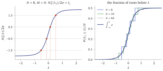
How many values may $I_j$ take? Since $\theta_n(\pm\infty)=\pm\pi$ , the function (16.2) runs from $-(N-M)\pi/N$ to $+(N-M)\pi/N$ , so $N\zeta/2\pi$ sweeps an interval of length $N-M$ .

Proposition 16.1 (The vacancy count). For $M$ finite real roots there are exactly $\#\{\text{vacancies}\}=N-M$ (16.3) allowed values of $I$ : the $N-M$ elements of $\Z+\tfrac{N-M+1}2$ with $\abs I\le\tfrac{N-M-1}2$ . If moreover the roots are pairwise distinct and $\zeta$ is strictly increasing, they occupy $M$ distinct ones and $N-2M$ are left as holes.

Proof. The allowed values are those strictly inside the range of $N\zeta/2\pi$ , an interval of length $N-M$ centred at $0$ ; the lattice $\Z+\tfrac{N-M+1}2$ meets its interior in $N-M$ points, symmetric about $0$ (Lecture 10 checked the endpoints: $I=\pm\tfrac{N-M+1}2$ belongs to a root at infinity). A strictly increasing $\zeta$ takes each value at most once, so pairwise distinct roots carry $M$ distinct values of $I$ ; subtracting them leaves $N-M-M$ .

Remark 16.2 (Monotonicity is a hypothesis, not a theorem). Distinct roots need not carry distinct quantum numbers: at $N=22$ two real roots of a genuine eigenstate share $I=\tfrac{19}2$ , with $\zeta'<0$ between them (the tutorial). So the second sentence of Proposition 16.1 is a hypothesis about the branch one is on — the branch this lecture uses, where $\zeta'>0$ . Lecture 10 was careful for the same reason.

Three consequences are worth naming at once, because Lecture 17’s excitations rest on them. On that branch, $M=N/2$ leaves no holes at all: the roots fill every vacancy. $M=N/2-1$ leaves two. And $N-2M$ is even for every $M$ when $N$ is even, so on an even ring holes are created in pairs; a single hole needs odd $N$ .

The limit

Now let $N\to\infty$ with $M/N$ fixed and suppose the roots and the holes fill out densities: the number of roots in $[\lambda,\lambda+\dd\lambda]$ is $N\rho(\lambda)\dd\lambda$ , the number of holes $N\rho_h(\lambda)\dd\lambda$ . Then $\tfrac1N\sum_l\theta_2(\lambda-\lambda_l)\to\int\theta_2(\lambda-\mu) \rho(\mu)\dd\mu$ , and $N\zeta/2\pi$ increases by one across every vacancy, so $\zeta'/2\pi$ is the density of vacancies — roots and holes together. Differentiating (16.2) gives the lecture’s equation.

Theorem 16.3 (The root-density equation). Write $a_n(\lambda)=\theta_n'(\lambda)/2\pi =\dfrac1\pi\,\dfrac{n/2}{\lambda^2+n^2/4}$ . Under the assumption above, $\rho(\lambda)+\rho_h(\lambda) =a_1(\lambda)-\int_{\R}a_2(\lambda-\mu)\,\rho(\mu)\,\dd\mu .$ (16.4)

proved from the assumption; for the assumption as the sources make it see Takahashi §§3.3–3.4 and Korepin–Bogoliubov–Izergin §§I.2–I.3

The assumption is an interchange of limits, and it is not proved here: say so aloud. What is assumed is that the chosen solutions of (16.1) converge, that their empirical measure has a density, and that the convergence is good enough to pass inside the integral. It is the subject’s standard working hypothesis, tested numerically rather than proved; Figure 16.2 is one such test.

One equation, two models — and a sign

Lecture 11 wrote the Lieb–Liniger equations in the same shape (11.11), $k_jL+\sum_l\theta(k_j-k_l)=2\pi I_j$ with $\theta(k)=2\arctan(k/c)$ . Both models are therefore instances of $L\,p_0(\lambda_j)+\sum_l\varphi(\lambda_j-\lambda_l)=2\pi I_j, \qquad \rho+\rho_h=\frac{p_0'}{2\pi} +\frac1{2\pi}\int K(\lambda-\mu)\,\rho(\mu)\,\dd\mu, \qquad K=\varphi' ,$ (16.5) with $L$ the number of sites $N$ or the length of the box. The dictionary between them is $\begin{aligned} \text{XXX:}&\quad p_0=\theta_1, &\varphi&=-\theta_2, & K(\lambda)&=\frac{-2}{1+\lambda^2} ,\\[2pt] \text{LL:}&\quad p_0=k, &\varphi&=+\theta, & K(k)&=\frac{2c}{k^2+c^2} . \end{aligned}$ (16.6)

The two kernels have opposite signs, and every formula below inherits it: Lecture 10 measures a magnon by $\theta_1=\pi-k$ , which runs backwards against its momentum, and Lecture 11 a particle by $k$ .

16.3 The Heisenberg antiferromagnet

Take $J>0$ in $H=J\sum(\mathbf S_n\!\cdot\!\mathbf S_{n+1}-\tfrac14)$ and $N$ even. A Bethe state has $E=-\sum_j 2J/(4\lambda_j^2+1)$ — (10.16), and equally what $\ii\,\dd\ln\Lambda|_0$ gave in Lecture 15 (Proposition 15.10). Every term is negative, which suggests, without proving it (adding a root moves all the others), that the ground state carries as many finite real roots as it can. The largest $M$ is $N/2$ (Lecture 10: the Bethe states are highest weight), and by Proposition 16.1 that sector has exactly $N/2$ vacancies. The antiferromagnetic ground state fills all of them: it is the state with $M=N/2$ and no holes, a total singlet cited for the identification with the lowest level: Hulthén (1938); Takahashi §3.3; checked here by comparing the filled sea with exact diagonalisation at $N=8$ , and by diagonalising the $S^{z}=0$ sector at $N=8,12,16$ and checking its lowest level against $S^{z}=1$ . For odd $N$ the lowest level is made of spin- $\tfrac12$ multiplets — two of them for $N=3,\dots,9$ (Lecture 10), so that already at $N=3$ the lowest level is four-fold degenerate — and the thermodynamic limit is therefore taken along even $N$ .

No holes means $\rho_h\equiv0$ on the whole line, and (16.4) becomes a convolution equation on $\R$ : $\rho(\lambda)+\int_{\R}a_2(\lambda-\mu)\,\rho(\mu)\,\dd\mu=a_1(\lambda) .$ (16.7) A convolution on the line is a product after a Fourier transform, and the transform of $a_n$ is as simple as can be.

Theorem 16.4 (The ground-state density and energy). With $\hat f(\omega)=\int f(\lambda)e^{\ii\omega\lambda}\dd\lambda$ one has $\hat a_n(\omega)=e^{-n\abs\omega/2}$ , and (16.7) has exactly one solution in $L^1(\R)$ , $\hat\rho(\omega)=\frac{1}{2\cosh(\omega/2)}, \qquad \rho(\lambda)=\frac{1}{2\cosh\pi\lambda} .$ (16.8) Its energy per site is $e_0=\frac EN=-\int_{\R}\frac{2J}{4\lambda^2+1}\,\rho(\lambda)\,\dd\lambda =-J\ln 2 .$ (16.9)

Proof. The function $a_n$ is a Cauchy density of half-width $n/2$ , whose transform is $e^{-n\abs\omega/2}$ (a residue at $\lambda=\pm\ii n/2$ , according to the sign of $\omega$ ). Transforming (16.7), $\hat\rho\,(1+e^{-\abs\omega})=e^{-\abs\omega/2}$ , so $\hat\rho=1/(e^{\abs\omega/2}+e^{-\abs\omega/2})$ , which is (16.8); inverting, $\frac1{4\pi}\int_{\R}\frac{e^{-\ii\omega\lambda}}{\cosh(\omega/2)}\dd\omega =\frac1{2\cosh\pi\lambda}$ . If two $L^1$ solutions differed, the difference would have a continuous transform killed by $1+e^{-\abs\omega}>0$ , hence zero. 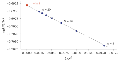For the energy, note that $2J/(4\lambda^2+1)=\pi J\,a_1(\lambda)$ , so by Parseval $e_0=-\pi J\int a_1\rho\,\dd\lambda =-\frac{\pi J}{2\pi}\int_{\R}\frac{e^{-\abs\omega/2}}{2\cosh(\omega/2)}\dd\omega =-\frac J2\int_0^\infty\frac{2e^{-\omega}}{1+e^{-\omega}}\,\dd\omega =-J\ln2 .$

Two checks: $\int\rho=\hat\rho(0)=\tfrac12=M/N$ , so the density knows the filling; and a finite chain’s roots really do distribute themselves like (16.8) (Figure 16.2), its energies converging to $-J\ln2$ along a straight line in $1/N^2$ (Figure 16.3) whose slope the reading explains.

Figure 16.2.

N=100

M=50

: the

50

Bethe roots of the ground state, solved from (16.1) by Newton’s method, as a histogram (left) and through their local spacing,

2/[N(\lambda_{j+1}-\lambda_{j-1})]

, on a logarithmic axis (right), against

1/(2\cosh\pi\lambda)

. The interior agreement is better than

2\%

N=100

Figure 16.3. Ground-state energy per site from exact diagonalisation,

N=8,10,\dots,20

, against

1/N^2

. The straight line through the largest four extrapolates to

-\ln 2

within

2\times10^{-5}

(square); its slope is

-0.8368

, within

2\%

of the asymptotic

-\pi^2/12=-0.8225

that the reading on finite size explains. The gap is the higher finite-size corrections, still visible at

N=20

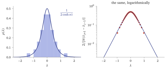
The sea of (16.8) occupies the whole rapidity line, and that is not a paradox: $k=\pi-\theta_1(\lambda)$ carries $\R$ onto the compact $(0,2\pi)$ , so an infinite sea of rapidities is a bounded set of momenta. Rapidity is the variable in which the equations are linear; momentum is the variable the experiment measures. The massless XXZ chain, $\abs\XXZ<1$ , has the same structure with $\pi$ replaced by an $\eta$ -dependent scale cited: Takahashi ch. 4; Franchini §4.4.

16.4 The Lieb–Liniger gas

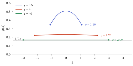
For the gas of Definition 11.2, $H=-\sum\partial_j^2+2c\sum_{i<j}\delta$ with $c>0$ on a ring of length $L$ , one thing changes: the energy $E=\sum k_j^2$ is a sum of positive terms, so the ground state should be the one whose quantum numbers sit as close to zero as they can: the consecutive block $I_j=-\tfrac{N-1}2,\dots,\tfrac{N-1}2$ of Lecture 11, which is the ground state at every $c>0$ cited: Yang–Yang (1969). Their roots are real and ordered (Proposition 11.4, Proposition 11.5) and fill an interval $[-q,q]$ : a Fermi sea of rapidities, with no holes inside and no roots outside. So (16.5) becomes an equation on a finite interval.

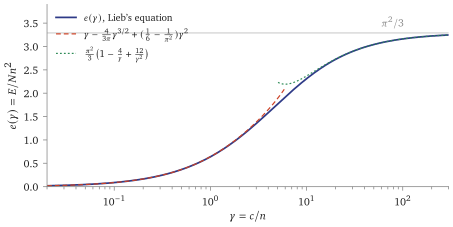
Theorem 16.5 (Lieb’s equation). In the ground state the rapidity density satisfies $\rho(k)=\frac1{2\pi} +\frac1{2\pi}\int_{-q}^{q}K(k-k')\,\rho(k')\,\dd k', \qquad K(k)=\frac{2c}{k^2+c^2}=-\ii\frac{\dd\ln S}{\dd k} ,$ (16.10) with $q$ fixed by the density, and then $n=\int_{-q}^{q}\rho\,\dd k,\qquad \frac EL=\int_{-q}^{q}k^2\rho\,\dd k,\qquad \gamma=\frac cn,\qquad \frac EN=n^2e(\gamma) .$ (16.11) The dimensionless $e$ depends on $c$ and $q$ only through $\gamma$ .

Proof. All but the last sentence is (16.5) with $p_0'=1$ , $\rho_h=0$ on $[-q,q]$ and $\theta'=K=-\ii\dd\ln S/\dd k$ (Proposition 11.1). For the last, substitute $k=qx$ , $g(x)=\rho(qx)$ : with $\alpha=c/q$ , $g(x)=\tfrac1{2\pi}+\tfrac1{2\pi}\int_{-1}^{1}\tfrac{2\alpha}{(x-y)^2+\alpha^2} g(y)\dd y$ , which involves $\alpha$ alone. Then $n=q\int g$ and $\gamma=c/n=\alpha/\!\int g$ , and $E/Ln^3=\int x^2g/(\int g)^3$ : both are functions of $\alpha$ alone, so the pair $(\gamma,e)$ traces one curve as $\alpha$ runs over $(0,\infty)$ , and that curve is a graph because $\gamma$ is strictly monotone: at fixed $c$ the Neumann series for (16.10) has a positive source and a positive kernel and converges, so enlarging $[-q,q]$ raises $\rho$ pointwise and adds interval; $n(q)$ is strictly increasing, $\gamma=c/n$ strictly decreasing in $q$ , hence strictly increasing in $\alpha=c/q$ .

Equation (16.10) has no closed-form solution, and this is where the subject turns numerical: a quadrature rule on $[-q,q]$ turns a Fredholm equation of the second kind into an $n\times n$ linear system. How large $n$ must be is set by the one parameter of the proof above. The kernel has width $c$ and the interval width $q$ , so the rule resolves it easily while $\alpha=c/q$ is of order one — twenty points give machine precision at $\gamma\approx1$ — and must be refined as $\alpha\to0$ , where the kernel becomes a spike. The tutorial shows how far a fixed rule can go wrong.

Figure 16.4. The Fermi sea of rapidities at three couplings, all at density

n=1

. At weak coupling the sea is narrow and

\rho

is peaked; as

\gamma

grows the sea widens towards

q=\pi n

and

\rho

flattens onto the free-fermion value

1/2\pi

The two limits

Proposition 16.6 (Impenetrable bosons are free fermions). As $\gamma\to\infty$ , $\rho\to1/2\pi$ on $[-q,q]$ with $q=\pi n$ , and $e(\gamma)\longrightarrow\frac{\pi^2}{3}, \qquad\text{i.e.}\qquad \frac EN\longrightarrow\frac{\pi^2n^2}{3} .$ (16.12) This is the ground-state energy per particle of free spinless fermions with $\varepsilon(k)=k^2$ at the same density.

Proof. In the scaled equation of Theorem 16.5 the kernel integrates to at most $2/\pi\alpha$ over $y\in[-1,1]$ , and $\alpha=c/q\to\infty$ , so $g\to1/2\pi$ uniformly. Then $n\to q/\pi$ and $E/L\to q^3/3\pi$ , whence $e=(E/L)/n^3\to\pi^2/3$ . For the free fermions the momenta are the $N$ allowed values nearest $0$ , spaced $2\pi/L$ , filling $[-\pi n,\pi n]$ at density $1/2\pi$ : the same integral.

At the other end $q\to0$ , the sea shrinks and the expansion is harder; Bogoliubov’s answer is $e=\gamma-\tfrac4{3\pi}\gamma^{3/2}+O(\gamma^2)$ sketched: mean field, then the zero-point energy of the Bogoliubov modes; cited for the coefficients, against $e=\tfrac{\pi^2}3(1-4/\gamma+O(\gamma^{-2}))$ at the other. Figure 16.5 shows both, and shows that neither survives $\gamma\sim1$ ; the reading carries the next orders.

Figure 16.5. The equation of state

e(\gamma)

from (16.10), with the weak- and strong-coupling series drawn past the range in which they are accurate so that they can be seen leaving the curve. There is no crossover scale:

\gamma\sim1

is the whole of it.

16.5 What it buys

Ground states in the thermodynamic limit: the antiferromagnet’s $e_0=-J\ln2$ in closed form (Theorem 16.4), and the gas’s equation of state $e(\gamma)$ at every coupling (Theorem 16.5).
One equation for both models, (16.5), with the kernel the derivative of the two-body phase: what Lecture 17 dresses and takes to finite temperature.
At infinite repulsion the gas’s ground state has the energy of free fermions (Proposition 16.6); Lecture 18 returns to free fermions.

16.6 Caveats, in one place

Status. Theorem 16.3 is proved from an assumption: that the chosen solutions converge and their roots fill out a density. It is the subject’s standard working hypothesis, tested numerically, not proved. Theorems 16.4 and 16.5 and Proposition 16.6 are proved given it. That the antiferromagnet’s lowest level is the filled sea, and the gas’s the consecutive block, is cited; the first is also checked against exact diagonalisation (at $N=8$ against the filled sea, and at $N=8,12,16$ by comparing the lowest levels of the $S^{z}=0$ and $S^{z}=1$ sectors).
Monotonicity is a hypothesis (Remark 16.2): distinct roots need not carry distinct quantum numbers, and the vacancy count’s second sentence assumes the branch on which they do.
The two ends of $e(\gamma)$ are asymptotic series; neither survives $\gamma\sim1$ , where only the integral equation does.

16.7 The two ends of $e(\gamma)$ , and the central charge

The asymptotics of §16.4 continue $e(\gamma)=\gamma-\frac{4}{3\pi}\gamma^{3/2} +\Bigl(\frac16-\frac1{\pi^2}\Bigr)\gamma^2+O(\gamma^{5/2}), \qquad e(\gamma)=\frac{\pi^2}{3}\Bigl(1-\frac4\gamma+\frac{12}{\gamma^2} +O(\gamma^{-3})\Bigr),$ (16.13) cited for the coefficients and the check script confirms each where Figure 16.5 draws it, the strong-coupling residual matching the known third coefficient in size and sign. It also pins the curve at an independently published point: by Hellmann–Feynman the kinetic and interaction energies are equal at $\gamma=4.3485(1)$ , where $e/2=0.82668(1)$ — and the solver used here gives $4.3486$ and $0.82668$ .

Figure 16.3 was a straight line in $1/N^2$ , and its slope is not an accident. A one-dimensional critical system in a box of $N$ sites has $E_0(N)=N e_0-\frac{\pi c\,v}{6N}+o(N^{-1}),$ (16.14) with $v$ the sound velocity and $c$ the central charge of the conformal field theory that describes its long distances cited: Blöte–Cardy– Nightingale and Affleck (1986). For the Heisenberg antiferromagnet the spinon dispersion $\varepsilon=\tfrac{\pi J}2\sin p$ of Lecture 17’s reading gives $\dd\varepsilon/\dd p=(\pi J/2)\cos p$ , so the speed of sound — its value as $p\to0$ — is $v=\pi J/2$ , and (16.14) predicts $E_0(N)/N=-J\ln2-\pi^2J/(12N^2)$ if $c=1$ . That is the slope in Figure 16.3. Reading it backwards, the numbers $-(E_0-Ne_0)\,6N/\pi$ fall from $1.596$ at $N=12$ to $1.583$ at $N=20$ by exact diagonalisation and reach $1.5721$ at $N=400$ by the Bethe equations, against $\pi J/2=1.5708$ : the central charge of the spin- $\tfrac12$ chain is $1$ , measured from its ground-state energies alone. The Lieb–Liniger gas gives $c=1$ the same way cited.

This is the cheapest known route to a central charge, and it is why the finite-size Bethe equations — solvable to machine precision at $N=400$ — are a standard instrument rather than a curiosity.

16.8 Solving Lieb’s equation

Theorem 16.5 is a Fredholm equation of the second kind, and the Nyström method turns it into linear algebra. Choose an $n$ -point Gauss–Legendre rule on $[-1,1]$ , scale it to $[-q,q]$ as $k_i=qx_i$ , $w_i\mapsto qw_i$ , and impose (16.10) at the nodes: $\Bigl(\delta_{ij}-\frac{w_j}{2\pi}K(k_i-k_j)\Bigr)\rho_j=\frac1{2\pi}, \qquad n\approx\sum_iw_i\rho_i,\qquad \frac EL\approx\sum_iw_ik_i^2\rho_i .$ (16.15) The kernel is analytic in the separation, so for a fixed $\alpha=c/q$ the rule converges faster than any power of $n$ : at $\gamma\approx1$ , $n=20$ already gives machine precision. But the constant in front of that statement is $\alpha$ , and the rule resolves a spike of width $\alpha$ only when $n$ is large compared with $1/\alpha$ . Measured against an $n=1600$ reference:

$q/c$	$\gamma$	$n=10$	$n=40$	$n=200$
$0.1$	$29$	$2\cdot10^{-13}$	$2\cdot10^{-13}$	$2\cdot10^{-13}$
$1.3$	$1.2$	$6\cdot10^{-7}$	$3\cdot10^{-13}$	$3\cdot10^{-13}$
$20$	$9\cdot10^{-3}$	$7\cdot10^{2}$	$0.7$	$6\cdot10^{-8}$
$200$	$10^{-4}$	$6\cdot10^{6}$	$2\cdot10^{5}$	$5\cdot10^{3}$

At the last row the computed density is not merely inaccurate: it goes negative, which the true one cannot (the Neumann series has a positive source and a positive kernel). Always run $n$ against $2n$ . A rule that is exact to machine precision in one regime can be useless two decades away, and nothing in the output says so.

One more subtlety: the nodes never reach $\pm q$ , so any quantity wanted at the edge — the chemical potential of Lecture 17, or the sound velocity — must be evaluated by putting $k=q$ back into the integral equation rather than by extrapolating the nodes. Interpolating with the linear rule that comes to hand put $\mu$ wrong in the fourth decimal, where the integral equation gives it beyond the sixth; a high-order interpolant through all the nodes loses nothing. The lesson is not that interpolation is bad but that the edge value is free — the equation already evaluates there.

The pair that shares a quantum number. Remark 16.2’s counterexample is worth meeting. At $N=22$ , $M=2$ , $\lambda_1=2.228461914574\ldots,\qquad \lambda_2=2.372786474870\ldots, \qquad I_1=I_2=\tfrac{19}2 ,$ (16.16) solve (16.1) to forty digits, and Lecture 10’s two-magnon wavefunction built on them is a genuine eigenvector: $\norm\Psi^2=5.7312$ and $\norm{H\Psi-E\Psi}/\norm\Psi=10^{-14}$ at $E=-0.1808904556\,J$ . Between the two roots $\zeta'=-4.6\times10^{-4}$ . Such pairs first appear at $N\approx21.9$ , which is why nothing at the $N\le20$ of Figure 16.3 could have found one: when a claim quantifies over all $N$ , test the smallest $N$ at which its failure mode is known to appear, not the largest $N$ the machine allows.

To get $e(\gamma)$ one does not solve for $q$ at fixed $\gamma$ : by the scaling in the proof of Theorem 16.5 it is easier to set $c=1$ , sweep $q$ , and read off the pair $(\gamma,e)=(1/n,\,(E/L)/n^3)$ . The curve of Figure 16.5 is $260$ such solves and takes about a second.

The same solve answers a question that looks harder. By Hellmann–Feynman the interaction energy is $\langle 2c\sum\delta\rangle=c\,\partial E/\partial c$ at fixed $N,L$ , so per particle it is $n^2\gamma e'(\gamma)$ and the kinetic energy is $n^2(e-\gamma e')$ . They are equal when $e=2\gamma e'$ , i.e. when the slope of $\ln e$ against $\ln\gamma$ is $\tfrac12$ ; the same solves, with the slope taken by a centred difference and set to $\tfrac12$ by bisection in $q$ , put that at $\gamma=4.3486$ with $e/2=0.82668$ , against the published $\gamma=4.3485(1)$ and $0.82668(1)$ cited: Caux, The Bethe Ansatz (integrability.org), the Lieb–Liniger ground state. A benchmark with two independent digits is worth more than a plausible-looking curve: this one is what fixed which power of $n$ the normalisation (16.11) carries.

Summary

Densities (Theorem 16.3): with roots and holes filling out densities, $\rho+\rho_h=a_1-a_2*\rho$ for the chain; both models are one equation (16.5), with kernels of opposite sign.
The antiferromagnet (Theorem 16.4): no holes, $\rho=1/(2\cosh\pi\lambda)$ by Fourier transform, and $e_0=-J\ln2$ .
The gas (Theorem 16.5): a Fermi sea of rapidities on $[-q,q]$ , Lieb’s equation, and $e(\gamma)$ , which tends to the free-fermion $\pi^2/3$ as $\gamma\to\infty$ (Proposition 16.6).
Next: Lecture 17 dresses the densities, finds the excitations, and heats the gas.

References

M. Takahashi, Thermodynamics of One-Dimensional Solvable Models, Cambridge University Press (1999), §3.3 (Hulthén’s solution); V. E. Korepin, N. M. Bogoliubov and A. G. Izergin, Quantum Inverse Scattering Method and Correlation Functions, Cambridge University Press (1993), §§I.2–I.3 (the counting, the thermodynamic limit, Lieb’s equation); F. Franchini, An Introduction to Integrable Techniques for One-Dimensional Quantum Systems, Springer (2017), chapter 2 and §§3.4–3.6, §4.4; E. H. Lieb and W. Liniger, Phys. Rev. 130 (1963) 1605; C. N. Yang and C. P. Yang, J. Math. Phys. 10 (1969) 1115; L. Hulthén, Ark. Mat. Astron. Fys. 26A (1938) 1. Finite size: H. W. J. Blöte, J. L. Cardy and M. P. Nightingale, Phys. Rev. Lett. 56 (1986) 742, and I. Affleck, ibid. 746.

The whole bibliography, lecture by lecture →

The thermodynamic limit: densities and ground states

What this lecture does

16.1 The question