12.1 The question
Lecture 0 showed three Toda particles leaving a collision with the momenta they came in with, rearranged, and promised the reason. So the question is
what does integrability do to scattering: when particles meet on a line and fly apart, what is conserved?
The answer: the set of momenta, which are the eigenvalues of the Lax matrix (Theorem 12.2), and the scattering map is a product of two-body maps, one per pair; for three particles the two ways of composing them agree (Figure 12.6). The worked example is two particles, in closed form (Proposition 12.1).
12.2 FPUT, and the Toda potential
Lecture 0 told the story of the Fermi–Pasta–Ulam–Tsingou chain, whose spring energy (0.2) is weakly nonlinear and whose energy came back to the lowest mode instead of spreading (a reading at the end recalls it).
In 1967 Toda looked for a spring law for which the chain has exact periodic nonlinear waves, trying elliptic functions as the nonlinear analogue of sines, and found the exponential (Toda, §2.1). With the constants set to one and , (12.1) which to cubic order is the FPUT spring (0.2), with (Figure 12.1). Compressed () it is a steep exponential wall; stretched, it softens to the constant force of the linear term.
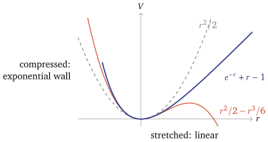
For a ring of springs the linear terms add up to the circumference, a constant, and can be dropped; the result is the Toda ring of Lecture 9, whose Poincaré section is Figure 7.5. For an open chain nothing holds the ends, and we drop the linear terms by fiat.1 What is left is the open chain of Lecture 8, (12.2) unit masses on a line, each repelled by its neighbours (Figure 12.2). The repulsion is felt only when particle comes close to, or overtakes, particle . So the open chain has no FPUT oscillations: its particles fly apart. It is a nonlinear many-body system simple enough to take apart completely.

It is Lecture 9’s Toda ring with its closing spring removed, and its Lax matrix is the tridiagonal one of Proposition 8.3.
12.3 Two particles in closed form
Take : . The mean momentum is conserved, and the centre of mass moves at the constant speed . The relative coordinate obeys and since , the energy of the relative motion is (12.3) It is positive because is, and it fixes . Particle starts behind particle (, where the potential is negligible) and approaches at relative speed ; the wall stops it at and sends it back.
Proposition 12.1 (The two-particle chain). Every solution with is, for some and a choice of origin, (12.4) Its properties:
- (a)
runs from to : the momenta are exchanged, from to .
- (b)
At every time the eigenvalues of are : the asymptotic momenta, and .
- (c)
With , as and , and the same with and the signs of reversed for the other pair. The straight line carrying the momentum is displaced by , the one carrying by .
Proof. Differentiating (12.4), , and . Every solution has exactly one turning point: , and cannot stay positive, since then increases and ; likewise backwards in time. A solution is fixed by its energy and the time of its turning point, where and , and (12.4) has both free. (a) follows. For (b), and by (12.3), so the characteristic polynomial is for all . For (c), use : then , and as , as .
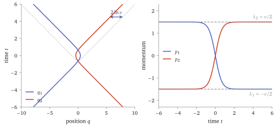
scripts/figures/toda_two_body.py, which checks (12.4) against a direct integration and the spectrum at every step).Read Figure 12.3 as a scattering experiment. In the far past there are two free particles with momenta , the faster one behind; in the far future, two free particles with the same two momenta, the faster one in front. Following the momentum rather than the particle, it is as if they had passed through each other, except that each straight line is displaced: the fast one by , a time delay when . This displacement is the classical counterpart of the two-body phase shift of the delta gas in Lecture 11. For its sign reverses: slow particles turn round while still far apart, and the momentum is handed forward across the gap.
12.4 General : elastic, non-diffractive scattering
For particles the general solution has determinant formulas (Moser; Babelon–Bernard–Talon, §4.8), which we omit: the asymptotics are all we need.
Theorem 12.2 (Moser cited). For every solution of the open Toda chain, as , and each particle moves asymptotically on a straight line: and . With the eigenvalues of , (12.5) The line carrying arrives on particle and leaves on particle , displaced by (12.6)
Given the separation, (12.5) is one line. If then every and . Eigenvalues depend continuously on the matrix and do not change in time, so is the spectrum . The separation fixes the order: as needs , so the outgoing momenta increase along the chain, and as they decrease. This is what the eigenvalues of mean, which is what Figure 8.3 was hinting at: they are the momenta the particles have when they are free. The separation and (12.6) are Moser’s (1975, pp. 480–481, in his normalisation; Toda, §3.10, gives (12.5) with halved); scripts/check-l9-algebra.py integrates in ours and finds both to within .
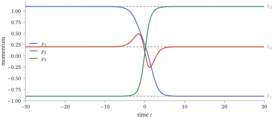
scripts/figures/toda_scattering.py, which asserts the spectrum constant to and both limits).Two words describe this (Figure 12.4). The scattering is elastic: the set of outgoing momenta equals the set of incoming ones, so each particle’s kinetic energy is handed on intact rather than shared. And it is non-diffractive: the outgoing momenta are not merely constrained by energy and momentum, which for would allow a continuum of outcomes; they are exactly the incoming ones, permuted. conserved eigenvalues leave room for nothing else.
Three particles: collisions in either order
Look at (12.6) term by term. The line carrying picks up from every faster momentum and from every slower one: exactly the two-body displacements of Proposition 12.1, one per pair, added. The total depends on the eigenvalues only. In particular it is the same whichever pair the incoming data bring together first.
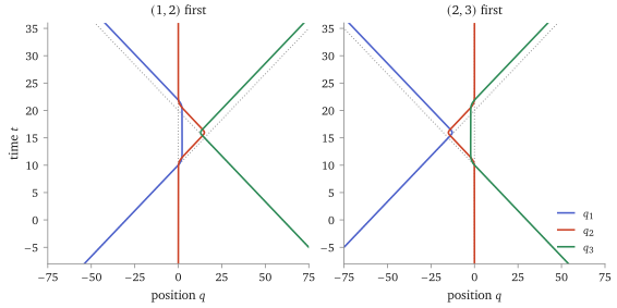
scripts/figures/toda_three_body.py, which asserts it; the check script also runs a genuine three-body collision and gets the same).Figure 12.5 makes it concrete. With incoming momenta on particles , started well apart, the run looks like three pairwise exchanges of momentum, which reverse the order, in the order or . The forces never switch off, so the exchanges are only nearly separate; the net result, (12.6), is exact. The two runs start from different incoming lines and look different throughout, but each outgoing line is displaced from its own incoming line by the same amount in both. Written as permutations of the three momentum lines, (Figure 12.6), and the displacements respect it.
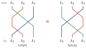
This is the concrete content of the phrase factorised scattering: the -body scattering map is a product of two-body maps, one per pair, taken along a route of crossings of adjacent lines from the incoming order of the lines to the outgoing one, and every such route gives the same map. The general theorem, that the -body scattering map of the open chain factorises this way, is Moser’s cited. It is a statement about the asymptotic motion: the particles scatter as if they met in pairs, although for more than two of them can interact at once. What we have seen is the two-body map in closed form and the three-body composition checked. Its quantum form is Lecture 11’s and Lecture 13’s: the two-body S-matrix has a phase whose derivative gives the packet displacement, and the braid relation becomes the Yang–Baxter equation.
12.5 What it buys
The meaning of the Lax eigenvalues: the momenta the particles carry when they are free, which is what Lecture 0’s collision figure showed.
Scattering without diffraction, the second face of integrability: -body scattering only permutes the momenta and shifts each line by a sum of two-body shifts.
The classical shadow of Part II’s key structures: the two-body shift against Lecture 11’s phase, and the braid relation, which with matrices at the crossings is Lecture 13’s Yang–Baxter equation.
12.6 Caveats, in one place
Status. Proposition 12.1 is proved. Moser’s theorem, the separation of the particles and the -body displacements (12.6), is cited; given the separation, the identification of the outgoing momenta with the eigenvalues of is one line. That the -body scattering map is a product of two-body maps is Moser’s too, a statement about the asymptotic motion, not a claim that the particles meet only in pairs; here the three-body composition is checked numerically.
A classical counterpart, not a limit, for the delta gas: classical point particles with a contact interaction show no displacement at all (Sutherland §4.2).
The linear terms of the spring are dropped by fiat on the open chain; the end particles go to infinity, where they would be an infinite constant.
The open chain’s own integrability is not used here, only its Lax matrix (Lecture 8) and Moser’s theorem. Its proof, and the reason its fibres are not compact, are in Lecture 9’s readings.
12.7 FPUT, recalled
In 1955 Fermi, Pasta, Ulam and Tsingou put a chain of masses joined by weakly nonlinear springs on a computer, with spring energy (12.7) the extension of the spring. They started it with all the energy in the lowest normal mode and expected the nonlinearity to share it out among all the modes. It did not: the energy wandered into a few neighbouring modes and came back, almost completely (Figure 1). A system that behaves this regularly is behaving as if it had more integrals than energy.
12.8 Why the open chain’s fibres are planes
Lecture 9’s readings prove the open chain Liouville integrable and each connected component of its level sets a cylinder (Corollary 9.24), with the number of periodic directions left open. The scattering picture settles it.
Proposition 12.3 (The fibres are planes sketched). In Corollary 9.24, : every is diffeomorphic to .
Proof (sketch). A stabiliser element means that the flow of returns every point of to itself at time ; in particular it returns the points of a trajectory at late times. There, by Theorem 12.2, the particles are far apart and . By (9.20) then moves particle at the speed , ; its speed is bounded on (proof of Proposition 9.23), so in unit time the particles stay far apart and the momenta barely change. Returning in time forces for every , hence and by the Vandermonde argument of Theorem 9.20. The stabiliser is trivial.
On a torus the commuting flows have a full lattice of periods, even though a single irrational flow need never return (Figure 5.2). On the open chain’s fibre no combination of the flows ever returns; the proof used the physical flow of , whose late-time configurations are free particles moving apart. In effect is coordinatised by the incoming offsets of Theorem 12.2, while the asymptotic momenta are fixed on it (Figure 12.7). They are the integrals, and they are also the obstruction: as long as they are distinct, the particles separate.
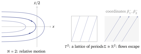
Close the chain into a ring and this changes. The whole ring can still drift (the flow of is still a translation), but the particles can no longer separate. Once the total momentum is fixed and the common translation split off, the relative level sets are compact, and each regular connected component is a torus , whose actions are read off a curve. That is Lecture 9.
Summary
- The model: the Toda spring is FPUT’s to cubic order; the open chain (12.2) is the Toda ring without its closing spring.
- Two particles (Proposition 12.1): the momenta are exchanged, they are the eigenvalues of at every time, and each momentum line is shifted by .
- particles (Theorem 12.2, cited): the outgoing momenta are the incoming ones, permuted, and the shifts are sums of two-body shifts (12.6): elastic, non-diffractive scattering.
- Three bodies: the two ways of composing the pairwise scatterings give the same shifts, the braid relation of Figure 12.6.
- Next: Lecture 13 asks what makes factorised scattering consistent when the particles carry a label, and finds the Yang–Baxter equation.
Worked in the tutorial: Exercise Sheet 12.
References
J. Moser, in Dynamical Systems, Theory and Applications, Lecture Notes in Physics 38 (1975) 467; Toda, Theory of Nonlinear Lattices, §§2.1, 3.10; Babelon, Bernard and Talon, Introduction to Classical Integrable Systems, §4.8; Sutherland, Beautiful Models, §4.2.
Toda, §3.10, following Moser: the end particles are sent to infinity, where the linear terms are an infinite constant.↩︎