5.1 The question
Functions in involution have commuting Hamiltonian vector fields, whose flows commute where they are complete (Corollary 2.6), and at most independent functions can be in involution (Proposition 4.11). A system with of them has as many conserved quantities as it can have. So the question is
what do independent integrals in involution force the motion to be?
The answer, Theorem 5.7, concerns a connected component of a common level set on which the integrals are independent at every point. If that component is compact, the motion is a straight line on a torus; if it is not, but the flows on it are complete, it is a straight line on a cylinder. The worked example is the two-dimensional oscillator (Example 5.3), whose level sets with both energies positive are the tori of Example 4.15.
5.2 Independence and involution
A first integral of is a function with (Definition 2.3). Each one confines the motion to a level set of — near any point where , a hypersurface of dimension . With several first integrals we collect them into one map, (5.1) and the motion stays in the level set through its initial point. Two things can go wrong with such a collection, and each has a name.
Definition 5.1 (Independence). are independent at if are linearly independent at — equivalently, if the Jacobian matrix of has rank there. They are independent if this holds on a dense open subset of .
Independence at a point is what the implicit function theorem needs: if it holds at , then near the level set is a smooth submanifold of dimension , with tangent space (5.2) Asking for it only on a dense open set is deliberate: in every example it fails somewhere, and the places where it fails are the interesting ones.
Definition 5.2 (Involution). are in involution if for all .
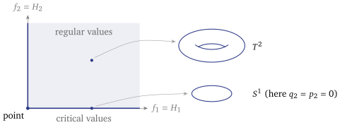
Example 5.3 (The two-dimensional oscillator). On take with , . The are in involution, since they involve disjoint variables. Their Jacobian is of rank unless one row vanishes, that is unless or . Those are two planes in , closed with empty interior, so the are independent. The level sets are pictured in Figure 5.1: the image of is the closed quadrant, over each interior point sits a torus, and over the edges — exactly where independence fails — the torus collapses to a circle or a point.
Each of the two conditions is easy to have without the other.
Example 5.4 (Independent but not in involution). For a particle in a central potential on , , the three components of are first integrals. So are three first integrals on a -dimensional phase space, and they are independent. They are not in involution: (5.3) and cyclically. Proposition 4.11 says three commuting independent functions is the most allows; three non-commuting ones are not the same thing.
5.3 Liouville integrable systems: the algebraic definition
Definition 5.5 (Liouville integrable). A Hamiltonian system with is Liouville integrable if there are independent functions in involution such that is a function of them, . Most often is one of them, .
By Proposition 4.11, is the most one can ask for.
Two remarks on the definition. First, is automatically a first integral of each , since it is built from functions that commute with ; and by the chain rule , so (5.4) Second, the functions are part of the data but not canonical: and in Example 5.3 define the same level sets.
Example 5.6 (Integrable systems we already own).
. Every with on a dense open set.
The -dimensional oscillator, with as in Example 5.3.
A central force in , with . Involution: for every , and by (5.3). Independence: the -components of are , all orthogonal to , while that of is ; so is independent of the other two wherever , and is independent of wherever is not parallel to . Both conditions fail only on the zero set of a nonzero polynomial.
5.4 The theorem, hypothesis by hypothesis
Theorem 5.7 (Liouville–Arnold proved modulo Lemma 5.10 and Theorem 1.9). Let be a symplectic manifold of dimension , and functions in involution. Fix , let be a connected component of the level set , and suppose
- (I)
are linearly independent at every point of ; and
- (C)
is compact.
Then:
is a smooth Lagrangian submanifold, invariant under the flow of every ;
is diffeomorphic to the torus , with angle coordinates defined modulo ;
for any , the motion on is , with a frequency vector that depends on only.
Deleting any one hypothesis gives a counterexample; three are exercises. The one to see now is compactness, the one the course will not have. The free particle on is integrable, with . At each component of its level set is a line , and the motion on it is not periodic: this is . When compactness fails but the flows on are complete, stage (iv) of the proof shows that a cylinder of this kind is the shape of the conclusion; without completeness there is no such classification. The Toda ring of Lecture 9 is the case the course needs it for.
5.5 The proof, in six stages
The proof turns commuting flows into an action of the group on , and then identifies with a quotient of . Groups acting on spaces have not appeared in the course so far, so stage (0) sets up the three words the proof uses.
Stage (0): an action of , its orbits and its stabiliser
Definition 5.8 (Action, orbit, stabiliser). An action of on a set is a family of maps , , with The orbit of is ; the action is transitive if some (hence every) orbit is all of . The stabiliser of is .
Lemma 5.9. is a subgroup of , the same for every point of the orbit of , and is a bijection from onto the orbit.
Proof. If then , and . If and , then — here we used : the group is abelian. Finally if and only if , i.e. .
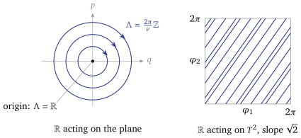
Two examples fix the words (Figure 5.2). The oscillator flow is an action of on the plane; the orbit of a point other than the origin is a circle with stabiliser , while the origin is its own orbit, with stabiliser all of . And on the torus the flow along the direction is an action of with stabiliser : the orbit is a copy of that never closes, winds densely (Lecture 6), and is still not the whole torus. One flow cannot fill a two-dimensional space; the proof uses flows on an -dimensional one.
Stage (i): is a Lagrangian submanifold
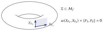
By (I) and the implicit function theorem, near each point of the level set is a smooth connected piece of dimension , which therefore lies in ; so is a smooth -dimensional submanifold with tangent spaces (5.2). The fields are tangent to it, because (5.5) At each point they are linearly independent, since and is injective (3.10). So the vectors are a basis of the -dimensional tangent space of at every point (Figure 5.3). On that basis , so vanishes on : is Lagrangian (Definition 4.10). Spent here: independence, and involution twice.
Stage (ii): complete commuting flows, hence an action of
The fields are tangent to , so they restrict to vector fields on the compact manifold , and by Proposition 1.7 they are complete there: each flow is defined on for all and maps to itself. By Corollary 2.6 these flows commute. Define (5.6) Then , and because the factors commute and each is a one-parameter group. This is an action of on . Spent here: compactness, for completeness, and involution, for commutativity.
Stage (iii): the action is transitive
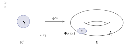
Fix and consider the orbit map , . Since the factors in (5.6) commute, any one of them may be put first, so The derivative of at every carries the standard basis of to a basis of the tangent space (stage (i)), so by the inverse function theorem is a local diffeomorphism: it maps a small ball about any diffeomorphically onto a neighbourhood of (Figure 5.4).
Consequently every orbit is open in . The orbits partition , so the complement of one orbit is a union of others and is open too; an orbit is therefore open and closed. is connected, so there is only one orbit. Spent here: independence (the local diffeomorphism), connectedness, and involution once more (the factors commute).
By Lemma 5.9, with now the same for every point of , (5.7)
Stage (iv): is a lattice of full rank
This is the step doing the most work, and it has two halves that must not be merged.
is discrete. Choose a ball about on which is injective (stage (iii)). If then , so . Translating, for any the ball contains no other point of , because . Every point of is isolated. Contrast , a subgroup with points arbitrarily close to : what excludes that here is independence, through the local diffeomorphism.
Lemma 5.10 (Discrete subgroups of cited). A discrete subgroup of is for some linearly independent , . (Arnold, §49 D, Lemma 3.)
Discreteness alone gives a cylinder, not a torus. Complete to a basis of . Then is well defined and bijective by (5.7), and a local diffeomorphism by stage (iii). A bijective local diffeomorphism is a diffeomorphism. So , and every from to is possible for a discrete stabiliser.
Compactness forces . is compact only if , and is compact. Hence has full rank and . Spent here: independence for discreteness, compactness for full rank — the second use of compactness, and the one that fails for the Toda ring of Lecture 9.
With (Figure 5.5) the two cases are a circle, with the period, and a line, , which is the free particle’s level set.
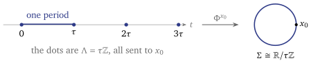
Stage (v): the period lattice and a basis of cycles
Definition 5.11 (Period lattice). The stabiliser of stage (iv) is the period lattice of . A basis of it gives basis cycles , , closed loops on .
A point comes back to exactly when , so the components of in the basis , times , are angles. Write for the matrix whose columns are the basis vectors, and set (5.8) These are the angle coordinates of Theorem 5.7: identifies with (Figure 5.6), and along the angle runs once from to while the others are constant.
Here is Lecture 3’s annulus again. Each is not a function on , only a function modulo , but is a well-defined -form, closed since it is locally of a function. It is not exact: whereas an exact form integrates to zero round every loop (Proposition 3.10). The torus carries independent closed non-exact -forms, detected by loops; Lecture 6 integrates over those same loops.
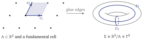
Stage (vi): straight-line motion, and what is left for Lecture 6
Let . On the coefficients in (5.4) are the constants , so , whose flow is : in the motion is . By (5.8), (5.9) That is conclusion 3 of Theorem 5.7, and it completes the proof.
One more fact is needed next time, and it is a consequence of stage (i).
Proposition 5.12 ( is closed on the torus). If is or a cotangent bundle, the restriction of to is a closed -form.
Proof. Restriction is pullback by the inclusion, and commutes with pullback (3.6). So , by Theorem 4.17 and stage (i).
So over a loop on is unchanged when the loop is deformed within (Corollary 3.13). That is what Lecture 6 needs to define the action variables and to show that, as varies, the angles (5.8) and the together form canonical coordinates on a whole neighbourhood of . The theorem as proved here is about one torus at a time; how the tori fit together as moves is Lecture 6’s business near one torus, and globally it can be subtle (optional lecture A).
One torus, two lattices
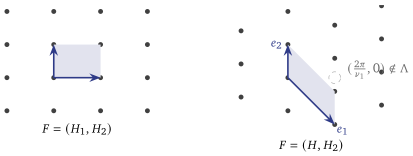
Example 5.13 (One torus, two lattices). Return to Example 5.3. The flow of turns the -th -plane clockwise at angular speed and leaves the other alone.
With , turns the planes through and , so , a rectangular lattice.
With , turns both planes and the second, so turns them through and . Now when and are both in , and a basis is Unless is an integer, : the lattice is not the product lattice of the first bullet (Figure 5.7).
The level set is the same torus in both cases, and the two lattices have the same cell area ; they describe the same torus with different generators of the action. The basis cycles are the same too: in both cases goes once round the first plane and once round the second.
By (5.9), with : the product lattice and give ; the second lattice and , , give again. The lattice depends on the choice of integrals; the motion does not.
5.6 What it buys
Tori, or cylinders. If the flows are complete on — which compactness guarantees but need not be what supplies it — stages (i)–(iv) give , and compactness is needed only to force . For the Toda ring, whose level sets are not compact, Lecture 9 proves completeness separately and finds .
Angles and cycles. The period lattice gives angle coordinates, basis cycles and a frequency vector (5.9); and, in or a cotangent bundle, is closed on the torus (Proposition 5.12). Lecture 6 integrates it over the cycles to get the actions, and completes the angles to canonical coordinates.
5.7 Caveats, in one place
Status. Theorem 5.7 is proved modulo the cited Lemma 5.10 and Theorem 1.9. Stage (ii) also uses Corollary 2.6 on . On and on cotangent bundles, where every cotangent chart is canonical (Theorem 4.17), the coordinate proof of Lecture 2 gives it. On a general symplectic manifold it rests on the Jacobi identity for the bracket of and the second proof of the engine, both proved in readings (Lecture 4, Lecture 2).
Independent on a dense set, or on all of . The definition allows the integrals to be dependent somewhere; the oscillator’s are, on two planes. The theorem applies only to the components of level sets on which they are independent at every point.
One torus at a time. The theorem is about one level set. How the tori fit together as varies is Lecture 6’s business near one torus; globally it can be subtle (optional lecture A).
Summary
- The definition is algebraic: independent functions in involution on a -dimensional phase space, with a function of them (Definition 5.5).
- The theorem (Theorem 5.7): a compact connected component of a level set, on which the differentials are independent, is a Lagrangian torus , and the motion on it is .
- The proof: tangent commuting flows, complete by compactness, give an action of ; independence and connectedness make it transitive, with a discrete stabiliser ; the quotient is , and compactness forces .
- The period lattice gives angles, basis cycles and frequencies (5.9); in or a cotangent bundle, is closed on the torus (Proposition 5.12).
- Next: Lecture 6 integrates over the basis cycles, and finds canonical action–angle coordinates near the torus.
Worked in the tutorial: Exercise Sheet 5.
References
Arnold, Mathematical Methods of Classical Mechanics, §49 (the theorem and its proof; Lemma 2 of §49 C is our stage (iii), Lemma 3 of §49 D our Lemma 5.10); Babelon, Bernard and Talon, Introduction to Classical Integrable Systems, ch. 2 (the theorem, and the examples). Conventions. Arnold writes , the negative of ours; nothing in this lecture depends on the sign of , since every use of it is a statement that something vanishes.