Lecture 3
The exterior derivative, Stokes, and the symplectic form
Course map: G1, step 3 of 9. Calculus on forms, and the one -form mechanics is built on. The exterior derivative tells a closed form from an exact one. Stokes’ theorem, cited, then shows that the integral of a closed -form round a loop depends only on the loop’s class, which is what will make the action variables of Lecture 6 well defined. The second half names the symplectic form, a closed, non-degenerate -form, and checks that its sign convention gives Hamilton’s equations.
3.1 The question
Lecture 2 gave a type, a -form, and left two requirements on the loop integral (2.8) open: it must not change when the loop is reparametrised, and it must not change when the loop is deformed. So the question of this lecture is
when does the integral of a -form round a loop depend only on the loop’s class — and what structure on phase space does come from?
The answer to the first is closedness, with Stokes’ theorem (Corollary 3.13). The answer to the second is the symplectic form , of which is a primitive up to sign (§3.6).
3.2 The exterior derivative
We have on functions. Extending it to forms of every degree is what turns this algebra into a calculus.
Definition 3.1 (Exterior derivative). On a -form (a function), is Definition 2.8. On a -form , (3.1) and in general acts on by differentiating each coefficient and wedging of it on the left. It raises degree by one and obeys the graded Leibniz rule (3.2)
The formula is written in coordinates, so it is fair to ask whether a different chart would give a different answer. It would not: is characterised by (3.2), by agreeing with Definition 2.8 in degree zero, and by , and those three conditions mention no coordinates. We take the characterisation on trust (cited; da Silva, §6) and use the formula.
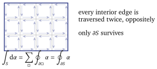
In the plane, for , (3.1) gives (3.3) using and . Evaluated on a small parallelogram, is the circulation of around its boundary (Figure 3.1). That reading is Stokes’ theorem in miniature, and §3.4 does no more than add such squares up.
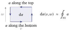
Theorem 3.2 (). for every form .
Proof. It is enough to check it on a function, since the general case follows by (3.2) and . With , Now split the double sum into the pairs . Within each pair the coefficient is symmetric in because mixed partials of a smooth function commute, while is antisymmetric by (2.13). Within each pair the two terms are equal and opposite, so the sum vanishes pair by pair.
Definition 3.3 (Closed, exact). A -form is closed if , and exact if for some -form .
Theorem 3.2 says exact closed. The converse is the interesting direction, and it is local.
Theorem 3.4 (Poincaré lemma cited). A closed form on a ball — or on any region that can be smoothly contracted to a point — is exact. (da Silva, §6; Arnold, §36.)
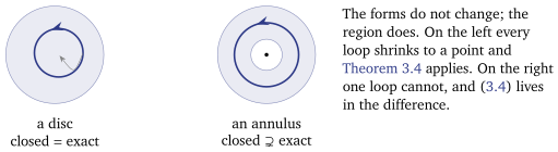
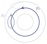
Everything this course does with forms lives in the gap between Theorem 3.2 and Theorem 3.4: closed and exact differ, and they differ only because of the shape of the region (Figure 3.2). §3.3 is the smallest example, and Lecture 6 is the payoff.
Grad, curl and div are one operator
In the forms of each degree have three, three and one independent components — and so do the classical vector operators. Writing in each degree reproduces them:
| degree | object | gives | classical name |
|---|---|---|---|
| a -form with components | |||
Read in this table, Theorem 3.2 is two familiar identities at once: and . They were never two facts. The dictionary is special to three dimensions — it relies on -forms and -forms both having three components — which is the reason the classical operators do not generalise and does. Phase space is -dimensional, so from here on only is available — which is why this comparison is worth making once and then leaving behind.
3.3 Closed but not exact: the annulus
Example 3.5 (The angle form). On the punctured plane — an annulus, for present purposes — put (3.4) Away from the origin this is smooth, and a two-line computation with (3.3) gives : it is closed.
In polar coordinates , which makes it look exact. It is not, and the reason is that is not a function on the annulus: continuing it once around the hole returns it increased by . The name is a name for the -form (3.4), not an assertion that something has been differentiated. To see this is not a quibble, integrate.
Proposition 3.6. is closed and not exact on .
Proof. Closedness is Example 3.5. For the rest, let be the unit circle traversed once anticlockwise, , . Substituting into (3.4) gives . If were for a function on the annulus, then by Proposition 3.10 below the integral around any closed curve would be . It is , so no such exists.
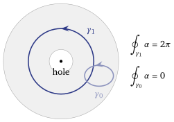
This is the smallest interesting fact in the lecture, and the one to remember. It is tempting to read Proposition 3.6 as bookkeeping. It is not:
The two halves do different jobs and neither can be dropped. Were exact on the torus, (2.8) would give for every cycle on it, by Proposition 3.10. The nonzero actions of the oscillator, the pendulum and the Kepler problem exist for the reason Figure 3.3 exhibits — a cycle that does not bound, and a closed form with no primitive along it.
3.4 Pullback, integration, and Stokes’ theorem
Pullback
Forms have one property vectors do not: they can be transported backwards along any smooth map, with no assumption that the map be invertible.
Definition 3.7 (Pullback). Let be smooth and let be a -form on . Its pullback is the -form on given by (3.5) where is the derivative of . For a -form, , and similarly in any degree.
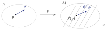
In practice pullback is substitution: if is given by , then , and one simply substitutes. Three rules follow, used later and the reason the formalism is worth its cost: (3.6) The first is the chain rule, and the second is the definition applied pointwise. The third follows from them for a -form, the case the deformation argument below uses: with and , the graded Leibniz rule (3.2) and give . The last rule — commutes with pullback — is what makes “closed” and “exact” coordinate-independent notions, and Lecture 4 will use the middle one to recognise canonical transformations as the maps satisfying .
Integration over a curve
Now the type-checking of §2.4 pays off.
Definition 3.8 (Line integral of a -form). For a smooth curve and a -form , (3.7)
Proposition 3.9 (Reparametrisation invariance). If is smooth, increasing and onto, then .
Proof (★). By the chain rule , so the integrand acquires exactly the factor that the substitution rule removes.
So the answer depends on the curve and its direction, not on the schedule. That was requirement 2 of §2.4, and Definition 3.8 met it by construction: a -form is precisely the kind of object whose integral over a curve needs no further data.
Proposition 3.10 (Fundamental theorem). . In particular for every closed curve.
Proof. by (2.9), and the one-variable fundamental theorem of calculus does the rest.
Proposition 3.10 is what Proposition 3.6 used, and it is also the statement that an exact form carries no information about loops. Everything interesting therefore lies with forms that are closed and not exact.
Stokes’ theorem
Theorem 3.11 (Stokes cited). Let be a compact oriented surface with boundary , carrying the induced orientation, and let be a -form defined on a neighbourhood of . Then (3.8) The same identity holds in every degree, for a -form on a -dimensional region. (Proof: da Silva, §6; Arnold, §36.)
We do not prove it. What we do instead is say exactly why it is true, because the mechanism is short and is the picture the rest of Part I uses.
Example 3.12 (Stokes on a rectangle, verified). Let and . By (3.3) and Fubini, after doing one integral in each term by the fundamental theorem of calculus. The four resulting boundary terms are exactly the four edges of , each with the sign the anticlockwise orientation gives it. That is (3.8) for a rectangle.
The payoff: integrals that depend only on the class of the loop
Corollary 3.13 (Deformation invariance). Let be a closed -form on a region , and let be a smooth deformation — a family of closed curves inside , running from to . Then
Proof. Pull back to the cylinder , where it is a -form on a -dimensional region. It is still closed, because commutes with pullback (3.6): . The boundary of is its two ends, the top with the orientation induced from and the bottom with the opposite one, so . By Theorem 3.11 applied on ,
This is requirement 3 of §2.4, discharged for closed forms: the integral of a closed -form depends on the loop only through its class. That is closed on the invariant tori, in or a cotangent bundle, is Lecture 5’s. An action variable is attached not to a curve but to a class of curves, and Lecture 5 will produce exactly such classes on an -dimensional invariant torus — the basis of cycles that Figure 3.6 shows for , and Lecture 6 will integrate over each of them in turn.
The worked example: the oscillator’s loop integral
Take the oscillator at unit frequency, , and its orbit : the circle of radius , traversed clockwise (§1.4), , for . Then (3.9) Stokes gives the same number without a parametrisation. The clockwise orbit bounds the disc it encloses, but with the orientation opposite to the one gives ; and . The two signs cancel: The loop integral is the area enclosed, and it is positive. Lecture 6 calls of it the oscillator’s action, .
3.5 The symplectic form
Lecture 2 built -forms, and §3.2 showed how to tell a closed one. The phase space of mechanics carries one closed -form with a special property, and the rest of Part I is built on it. One piece of notation first: a -form eats two vectors, and feeding it one leaves a -form.
Definition 3.14 (Interior product). For a -form and a vector at the same point, is the -form . The slot that fills is the first.
Definition 3.15 (Symplectic form, symplectic manifold). A -form on a manifold is symplectic if
it is closed: ; and
it is non-degenerate: at each point, if for every , then .
The pair is a symplectic manifold.
Condition 2 says that the linear map from to has zero kernel. The two spaces have the same dimension, so (3.10) A symplectic form converts vectors into covectors and back, with no choices made — the job an inner product does in Euclidean space, done by an antisymmetric object.
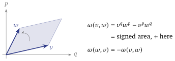
Example 3.16 (The standard symplectic form). On with coordinates , (3.11) by (2.12). Geometrically, is the sum over of the signed areas of the shadows of the parallelogram on in the -planes; for it is the signed area itself (Figure 3.7). It pairs each position only with its own momentum.
In matrix form, with vectors written as columns in the order , (3.12) It is closed because its coefficients are constant, and non-degenerate because .
The sign test, on one degree of freedom
The wedge order is not a matter of taste. Ask which satisfies on . By Definition 3.14 and (2.12), and matching with gives (3.13) Hamilton’s equations, both signs right; for the pendulum this is , . Had we written , the same computation would return and — both signs wrong. That is the whole reason for the order.
3.6 What it buys
The action variables can be defined. A closed -form integrates to the same number over any two loops that deform into one another (Corollary 3.13). On the invariant tori of Lecture 5, in or a cotangent bundle, is closed, and Lecture 6 integrates it over each torus’s independent cycles (Figure 3.6).
and are one object. On , by (3.1) and (2.13), so the standard symplectic form is exact, and closed by Theorem 3.2. The minus sign comes with the wedge order that the sign test fixed. Lecture 4 shows the same on every cotangent bundle, where needs no coordinates.
A symplectic form turns functions into flows. By (3.10), has exactly one solution , and on it is Hamilton’s vector field (3.13). Lecture 4 makes this the definition of on any symplectic manifold, and shows that it agrees with Lecture 2’s.
3.7 Caveats, in one place
Status. Three results are cited: that does not depend on the chart, the Poincaré lemma (Theorem 3.4), and Stokes’ theorem (Theorem 3.11). Deformation invariance (Corollary 3.13) is proved from Stokes, so it is proved modulo a cited theorem, and so is everything later that rests on it. Reparametrisation invariance (Proposition 3.9) is proved in a reading.
A deformation carries orientations. Corollary 3.13 needs a deformation, not merely two loops that together bound a region. The circle traversed anticlockwise and the circle traversed clockwise bound the annulus between them as point sets, yet the angle form (3.4) integrates to over the first and to over the second.
Summary
- The exterior derivative. (Theorem 3.2), so exact forms are closed. The converse holds on a ball (the Poincaré lemma) and fails on the annulus (Proposition 3.6).
- Integration. A -form integrates over a curve with no further data and independently of the parametrisation, and round any closed curve.
- Stokes (cited) gives deformation invariance: a closed -form integrates to the same number over loops that deform into one another (Corollary 3.13). That is what will make the action variables well defined.
- The symplectic form is a closed, non-degenerate -form. On it is , and its wedge order gives Hamilton’s equations with the right signs (3.13).
- Next: Lecture 4 shows that the bracket and the forms are one structure, and finds the shape the invariant tori will have: Lagrangian.
References
da Silva, Lectures on Symplectic Geometry, §1 (symplectic forms) and §6 (forms, , the Poincaré lemma, Stokes); Arnold, Mathematical Methods of Classical Mechanics, §§35–36 (integration of forms, Stokes), §37 (symplectic structures) and §44 (the action integral this lecture was built to support).
End of Lecture 3
The exterior derivative, Stokes, and the symplectic form
Lecture 3 · Contents
Keyboard
- → Space PgDn
- next screen, stopping before an equation, figure or statement it would cut
- ← PgUp
- previous screen
- ↓ ↑ wheel
- scroll freely
- Home End
- the start or the end
- S
- Full ↔ Spine, keeping your place
- T
- Think first on or off
- R
- reveal the next hidden proof
- C
- Core only on or off
- G
- contents: jump to a section or a statement
- + −
- text size
- D
- light or dark
- F
- full screen
- P
- pen on or off: draw on the text
- E
- erase the ink on the screen
- Z double-click
- enlarge an equation, figure or table; Z again for the next
- L
- laser pointer on or off
- B .
- blank the screen
- M
- move the toolbar: right, bottom, left, top
- ?
- this help
- Esc
- close a panel