Take $N$ equal masses in a row, joined by springs, with the two ends fixed. If the springs obey Hooke’s law the problem is linear and completely solved: the motion is a superposition of $N$ normal modes, the $k$-th a standing sine wave with frequency $$\omega_k=2\sin\frac{k\pi}{2(N+1)},\qquad k=1,\dots,N$$(0.1) (in units with mass and spring constant one). Each mode is a harmonic oscillator on its own. The energy in each mode is conserved separately: $N$ conserved quantities, one per mode. Start the chain in the lowest mode and it stays there for ever.

Now make the springs slightly nonlinear. With $r$ the extension of a spring, take the spring energy $$V(r)=\frac{r^{2}}2+\alpha\,\frac{r^{3}}3 ,$$(0.2) with $\alpha$ small. The modes are now coupled: the cubic term lets energy flow from one to another. What should happen seemed clear to Fermi (Toda, §1.1). The expectation, from statistical mechanics, was that a large system of coupled degrees of freedom, left alone, forgets everything about how it was started except its conserved quantities — here, only the total energy — and settles into thermal equilibrium, where on average every mode holds the same share of the energy. That is equipartition. The nonlinearity was put in precisely to let it happen, and the plan was to watch how long it took.

Fermi, Pasta and Ulam, with Mary Tsingou writing and running the programs on one of the first electronic computers at Los Alamos, integrated this chain with $32$ and with $64$ masses, all the energy in the lowest mode at the start (Toda, §1.1). The 1955 report thanked Tsingou for coding and running the computations; her decisive part was properly recognised, and her name added to the problem’s, only about fifty years later (Dauxois 2008). Figure 1 is the same experiment, integrated for these notes.

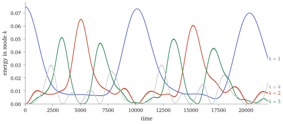
The energy did spread — into the next few modes, never into the rest — and then it came back. Not equipartition: a recurrence, the chain returning almost exactly to where it started, again and again.

It is not an artefact of the integration: in Figure 1 the total energy is conserved to a few parts in a million over the whole run, and the recurrence has been reproduced many times since (Toda, §1.1). What it says is that the chain behaves as though it had more conserved quantities than energy. Energy alone cannot stop the flow into the high modes: every way of sharing out the same energy is allowed by that one constraint. Something else is holding the motion back. The Hooke chain had $N$ conserved quantities and never forgot anything; the question FPUT raised is how much of that survives the nonlinearity.

Fifty years later the same question was asked of a quantum system, with atoms instead of a computer. Kinoshita, Wenger and Weiss (2006) trapped rubidium-87 atoms in an array of thin tubes made of laser light, each tube holding between $40$ and $250$ atoms and so narrow that the atoms can move only along it: a one-dimensional gas, with a harmonic trap along the tube. A short sequence of light pulses set each atom into a quantum superposition of moving one way and the other, so that the gas in each tube split into two clouds with opposite momenta. The two clouds then oscillate in the trap, passing through each other at its centre twice per period (Figure 2).

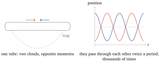
Two clouds of gas colliding head-on thousands of times should thermalise: the momentum distribution of the atoms should relax to a single thermal hump. It did not. After thousands of collisions the gas had not noticeably equilibrated; the two populations were still there. The name is the desk toy’s: a row of steel balls in which the momentum given to one end passes down the row and leaves at the other, over and over, without ever spreading out.

Both experiments watched a system of many interacting parts and waited for it to forget its starting point. Neither did. In statistical mechanics the only things a system is allowed to remember are its conserved quantities, and what thermal equilibrium means is that the energy (with total momentum and particle number, where they are conserved) is all it remembers. A system that remembers more, for as long as these did, is evidence of further constraints on the motion — exact conserved quantities, or approximate ones that hold for a long time. Integrability is the case in which there are enough exact ones to pin the motion down. The FPUT chain turns out to be close to such a case, and the cradle’s gas very close (§0.4 says how close, and on whose authority). So the question of the course is

For particles on a line, two lines of mechanics already answer the first half (§0.2). The second half is the course, laid out on one page in §0.3. It makes integrability precise twice, classically in Lectures 1–9 and quantum mechanically in Lectures 10–20, and comes back to both experiments: FPUT in Lecture 12, where the Toda chain’s spring turns out to be FPUT’s through cubic order, and the cradle in Lecture 20.

The Newton’s cradle already contains the key fact, and it takes two lines of algebra.

For particles that cannot pass through each other, only the exchange is possible. The conclusion needs equal masses. For masses $m_1\ne m_2$ the same two laws give $w_1=\big((m_1-m_2)v_1+2m_2v_2\big)/(m_1+m_2)$, and $w_1-v_2=(m_1-m_2)(v_1-v_2)/(m_1+m_2)$ is not zero: the velocities are reshuffled into new values. It also needs one dimension: in the plane, three conservation laws (two components of momentum, and energy) for four unknown velocity components leave a one-parameter family of outcomes, labelled by the scattering angle, and that is how a gas in two or three dimensions shares out energy.

So in one dimension, a gas of identical particles cannot change its set of velocities by two-body collisions at all. The list of velocities is merely handed from particle to particle. If the velocity distribution is to relax, something else has to do it: three particles close together at once.

For three equal masses the count changes. Momentum and energy are still two equations, but now for three unknown outgoing momenta, and two equations in three unknowns leave a one-parameter family. The family is a circle: with $P$ the total momentum, $$p_1^{2}+p_2^{2}+p_3^{2}=\frac{P^{2}}3+u^{2}+v^{2},\qquad u=\frac{p_1-p_2}{\sqrt2},\quad v=\frac{p_1+p_2-2p_3}{\sqrt6},$$ so fixed $P$ and fixed energy $E$ confine the outgoing momenta to the circle $u^{2}+v^{2}=2E-P^{2}/3$ (scripts/check-l0-algebra.py, group 3). The six rearrangements of the incoming momenta are six points on it. A generic three-body collision lands somewhere else on the circle, and the set of momenta changes. That is how a one-dimensional gas can thermalise.

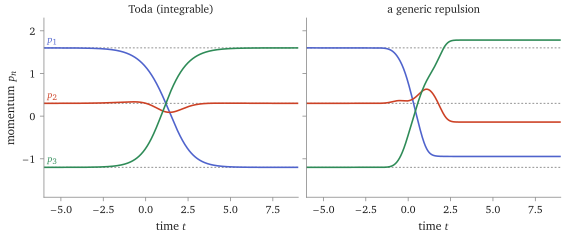
Figure 3 runs the experiment twice. On the right, a reasonable short-range repulsion; the three particles leave with new momenta. On the left, the Toda chain, an interaction chosen so that it has as many conserved quantities as particles — and the three particles leave with the momenta they came in with, rearranged, exactly as if they had met in pairs. Lecture 12 explains why. The chain carries a matrix, its Lax matrix, which changes in time but only in a way that keeps its eigenvalues fixed; long before and long after the collision it becomes diagonal, with the momenta on the diagonal. So the incoming and the outgoing momenta are both its eigenvalues (the separation of the particles, which this uses, is a cited theorem there). For such a system, in scattering, the rest of the argument goes through: no collision, of two particles or of three or of $N$, changes the set of momenta the particles carry away. A gas is harder, because its particles are never free for long and their momenta at any instant do change. What an integrable gas conserves instead are quantities that play the part of the asymptotic momenta (in Part II, the rapidities). In a uniform gas their distribution is conserved, which stops the gas relaxing to ordinary thermal equilibrium; in the trap of the cradle it moves, and to a good approximation keeps returning. Lecture 16 makes the distribution precise, Lecture 19 and Lecture 20 the ensemble it fixes, and Lecture 20 its motion in a trap. The atoms of the Newton’s cradle interact, to a good approximation, by point-like contact forces, and the one-dimensional Bose gas with point-like interactions is exactly such a system in its quantum form — the Lieb–Liniger gas of Lecture 11. Kinoshita, Wenger and Weiss themselves suggested this as the probable explanation.

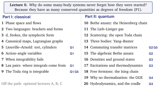
Proposition 0.1 and Figure 3 already hold the answer the course makes precise. A system that never forgets how it was started has conserved quantities beyond the energy. In the integrable case it has as many as it has degrees of freedom, and in one dimension they can be as simple as the set of momenta the particles carry. Figure 4 is the course on one page: two halves, five goals, and every lecture opens by saying where on this map it stands.

The five goals. A student who finishes the course can

1. prove a many-body system integrable from scratch, and say what that buys: the Toda chain on a ring (Lectures 1–9);

2. build a family of commuting quantum conserved quantities from one matrix, and diagonalise it: the Heisenberg spin chain (Lectures 10–15);

3. solve an interacting quantum gas exactly and take it to the thermodynamic limit: the Lieb–Liniger gas (Lectures 11, 16 and 17);

4. explain why an integrable system does not thermalise, and predict where it goes instead: a quench of the Ising chain, then a gas in motion (Lectures 18–20);

5. show that the quantum structure of G2 becomes the classical structure of G1 as $\hbar\to0$, on the quantum Toda chain (Lecture 14).

Five ideas carry them, and each lecture uses one or two:

1. Integrability is a count: as many independent conserved quantities, compatible with one another, as degrees of freedom. What it buys is free motion in the right variables (Lectures 5 and 6).

2. For the Toda ring and the Heisenberg chain the conserved quantities come as one family, the trace of a matrix that depends on an extra parameter, and they commute because of one local identity: classically in Lecture 9, quantum mechanically in Lecture 14.

3. Integrable scattering only rearranges momenta, and many-body scattering is a sequence of two-body events. Their consistency is one equation, the Yang–Baxter equation (Lecture 13); putting the particles on a ring then fixes each momentum by an equation of its own, a Bethe equation (Lectures 10–13).

4. With many particles the momenta become a density, fixed by one linear integral equation. That equation gives the ground state (Lecture 16), and dressing by it gives the excitations (Lecture 17). At a temperature one more equation, a nonlinear one, fixes how full each momentum is and gives the equation of state (Lecture 17). In a gas that flows, dressing gives the velocity at which each momentum travels, and the density of each momentum is carried along at that velocity: the hydrodynamics of Lecture 20.

5. What an integrable system conserves, it remembers: it relaxes, but to an ensemble that keeps every conserved quantity, not to a thermal state (Lectures 19 and 20).

How each lecture is built. Every lecture follows the same order: its question; only the definitions the question needs; one worked example on the course’s running model; the statement; its proof; what the result buys; the caveats, gathered in one section; and a summary pointing to the next lecture. Proved is the default and carries no mark. A result that is only sketched or cited is marked so where it is stated. Sections marked ★ are reading, and sections marked ▸ are tutorial; neither is lectured, and no core argument depends on them.

What is assumed: calculus, linear algebra (including eigenvalues and tensor products of matrices), ordinary differential equations, classical mechanics in Hamiltonian form, and quantum mechanics at the level of spin and perturbation theory. What is not: manifolds, differential forms, symplectic geometry, Lie groups, representation theory. Each is built, concretely, in the lecture that first needs it. What is not done: integrable field theories — solitons, the Korteweg–de Vries equation, the inverse scattering transform — which need this course first. The optional lectures A (quantum chaos and level statistics), B (the Calogero–Moser systems) and C (nesting and the Hubbard model) lie off the path.

• FPUT is not integrable. Its spring agrees with a Toda spring through cubic order, for every $\alpha\ne0$ (the tutorial at the end of this lecture), and the Toda chain with fixed ends is integrable (Toda, §2.10) cited. Numerical studies find that at low energy, and for very long times, the FPUT chain stays close to it (Benettin, Christodoulidi and Ponno 2013) cited. On that reading the recurrence is the shadow of the Toda chain’s conserved quantities. The course proves neither statement. It proves the Toda chain integrable on a ring (Lecture 9), and solves its scattering on an open line (Lecture 12).

• The cradle is only nearly integrable. The trap along the tube, and the tube’s finite width, break the integrability of the Lieb–Liniger description slightly. Why the gas still did not thermalise on the time scale of the experiment is Lecture 20’s business.

• In quantum mechanics, counting conserved quantities is not a definition. A Hamiltonian on a finite-dimensional space commutes with the projector onto each of its own eigenspaces, so commuting conserved quantities are never in short supply, and what “independent” should mean has no agreed answer (Caux and Mossel 2011). Part II therefore works with the two criteria of P3 and P2: scattering that only rearranges momenta, in the solutions of Lectures 10–13, and one commuting family from one matrix, for the Heisenberg chain in Lectures 14 and 15. The Ising chain of Lectures 18 and 19 is solved another way, by turning it into free fermions.

The FPUT computation was written up as a Los Alamos report in 1955 (Fermi, Pasta and Ulam, LA-1940). Mary Tsingou’s part — she wrote and ran the programs — was brought to light by Dauxois (2008), and the problem now carries her name. The first explanation came from the continuum. Zabusky and Kruskal (1965) replaced the chain by a partial differential equation, the Korteweg–de Vries equation, found numerically that its localised waves pass through one another and re-emerge unchanged, called them solitons, and read the recurrence through their motion (Toda, §§1.1 and 2.7). That line leads to the inverse scattering transform and to classical field theory, which this course leaves out. Toda (1967) went the other way: keep the lattice, and look for a spring law for which the chain has exact nonlinear waves. He found the exponential spring of Lecture 12, and the Toda chain turned out to be integrable. Whether the FPUT chain itself eventually equipartitions, and on what time scale, is still studied numerically, and the Toda chain is now the reference point for that question (Benettin, Christodoulidi and Ponno 2013).

The general Toda spring, with two constants $a$, $b$, is $$V_{\mathrm{T}}(r)=\frac ab\,e^{-br}+ar-\frac ab =\frac{ab}2\,r^{2}-\frac{ab^{2}}6\,r^{3}+O(r^{4}),$$ the constant chosen so that $V_{\mathrm T}(0)=0$; the linear terms cancel. Match it to $\kappa\big(\tfrac12r^{2}+\tfrac\alpha3r^{3}\big)$, the FPUT spring (0.2) with a spring constant $\kappa>0$. The quadratic terms give $ab=\kappa$ and the cubic terms $-ab^{2}/6=\kappa\alpha/3$, so $$b=-2\alpha,\qquad a=-\frac{\kappa}{2\alpha}.$$ For every $\alpha\ne0$ there is exactly one Toda spring that agrees with FPUT’s through cubic order. For $\alpha<0$ both constants are positive; with $\kappa=1$, $\alpha=-\tfrac12$ it is $e^{-r}+r-1$, the spring of Lecture 12. For $\alpha>0$, as in Figure 1, both are negative, and $V_{\mathrm T}(r)$ is the $\alpha<0$ spring with $r$ replaced by $-r$: the chain of Figure 1 is, to cubic order, a Toda chain with compression and extension exchanged (scripts/check-l0-algebra.py, group 4). The two springs part company at quartic order, and that difference is what makes FPUT a perturbation of Toda rather than Toda itself.