Lecture 18
Free fermions: the transverse-field Ising chain
Course map: P5 begins; the model of G4. Here is a chain of spins that looks interacting and is not. A change of variables due to Jordan and Wigner turns its spins into fermions and the Hamiltonian into a quadratic form; Fourier and Bogoliubov then diagonalise it completely. The lecture does this by hand, including the one step that short accounts drop: the chain splits into two sectors with different boundary conditions. The result is the model in which Lecture 19 proves relaxation to a generalised Gibbs ensemble.
18.1 The question
The chains and gases of Lecture 10, Lecture 11 and Lecture 15–Lecture 17 needed the Bethe ansatz because their particles scatter. Some chains only look as if they do. So the question is
which interacting-looking chains are secretly free, and how do you solve them completely?
The answer, for the transverse-field Ising chain: the Jordan–Wigner map (Theorem 18.3) makes it quadratic in fermions, sector by sector, and Fourier and Bogoliubov give its whole spectrum in both parity sectors (Theorem 18.6). The worked example is the chain itself, against exact diagonalisation (Figure 18.3).
18.2 The models
On a ring of sites, each carrying a spin with Pauli matrices , the transverse-field Ising model (TFIM) is (18.1) The first term wants neighbouring spins aligned along ; the second, the transverse field, wants every spin up along . The two do not commute, and that competition is the whole model. is even throughout. (For odd the momentum moves from one of the grids of §18.5 to the other; nothing changes in principle, but the bookkeeping does, and it is not treated.)
Two limits by inspection. At the ground state is with energy , and flipping one spin costs . At there are two ground states, all spins along or all along , energy ; the cheapest excitation of a ring is a pair of domain walls, each breaking one bond at cost , so in all. Between the limits something must happen, and the reading at the end finds it at .
The symmetry. Let (18.2) Each commutes with the field term and anticommutes with , so commutes with every bond (two anticommutations) and with . It is the spin flip , it squares to , and it splits the Hilbert space into an even sector and an odd sector . It exchanges the two ground states, so the combinations with a definite parity are their sum (even) and difference (odd).
18.3 Fermions
The algebra
Definition 18.1 (Fermionic modes). Operators on a Hilbert space satisfy the canonical anticommutation relations (CAR) if (18.3) where . The operator is the occupation of mode , and the fermion number.
Everything about these operators follows from (18.3). Taking in the second relation gives and : no mode can be created twice — Pauli’s principle. Then , so each has eigenvalues and , and the commute with each other.
Fock space. Suppose a unit vector , the vacuum, has for all . The vectors are eigenvectors of every , with exactly for the listed; they are orthonormal, their span is mapped to itself by every and , and the action there is fixed by the CAR alone. The order of the ’s matters only through a sign: . That sign is what makes fermions fermions, and it is where spins differ.
Spins are not fermions
On one site, and satisfy and : one spin is one fermionic mode, with empty and occupied. But on two different sites, and act on different tensor factors, so they commute; their anticommutator is . Spin flips on different sites are hard-core bosons: they exclude each other on a site and commute between sites. The fix has to supply a minus sign whenever two flips are exchanged, and it cannot be local.
18.4 The Jordan–Wigner map
Definition 18.2 (Jordan–Wigner). On spins, set (18.4) The product is the string; .

A fermion is a down spin, and the string counts how many fermions stand to the left (Figure 18.1): since on and on , (18.5) The strings cancel in because and acts on other sites than . The vacuum is , and the spin parity (18.2) is the fermion parity.
Proof. Everything rests on one fact about a single spin: (18.6) (, since outputs ; and , since it accepts only ). Same site. commutes with and , so and . Different sites, . Write with . The operators , , act on sites other than and commute with everything at site ; so and (18.6) gives . Replacing by , or by , changes nothing in the argument, which gives ; is the same with the names exchanged, and the remaining relations are adjoints. The converse is (18.4) multiplied by , and (18.5).
The Hamiltonian in fermions
The field term is immediate: . A bond between neighbours is almost as easy, because the strings of and differ by one factor.
Proposition 18.4 (Bonds and the boundary term). With ’s as in (18.4),
Proof. By Theorem 18.3, . First, the one-site identities and (because and ) give and . Bulk. , and commutes with , so which is (18.7). Boundary. Now the string is the whole chain but site : , and . So .
The boundary bond is the one term that is not a quadratic form in the ’s: it carries the parity of the whole chain. But commutes with , so on each sector it is a number, and there the boundary term is quadratic after all. Define in the even sector and in the odd sector. Then in both, (18.8) reads , the same form as the bulk, and (18.9) with : the fermions are antiperiodic in the even sector and periodic in the odd one. Each is quadratic, commutes with (every term changes by or ), and acts on all of Fock space. So the spectrum of is found in two steps: diagonalise and completely, then keep the even states of the first and the odd states of the second. The half thrown away is not part of the spin chain.
18.5 Fourier and Bogoliubov
Two grids of momenta
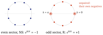
In each sector the fermions obey , so the plane waves that respect this are with : (18.10) with taken mod . (The names are borrowed from string theory, Neveu–Schwarz and Ramond, where the same two boundary conditions occur.) Both grids are symmetric under . The R grid contains and , which are their own negatives; the NS grid, for even , contains neither (Figure 18.2). In the sector’s grid set (18.11) The matrix is unitary, so the satisfy the CAR, and computed from (18.11) is automatically.
Proposition 18.5 (The Hamiltonian in momentum space). In each sector, with running over that sector’s grid, (18.12)
Proof. Substitute (18.11) and use on the grid. The field gives . Expanding the bond, . Hopping: , and with its conjugate this gives . Pairing: ; relabelling and using turns this into , and the last term is its conjugate.
The pairing term creates or destroys fermions two at a time, at and : the fermion number is not conserved, only its parity. So group the modes in pairs. For on the grid write , Collecting the terms of and in (18.12), and reordering , (18.13) where the second sum is present only in the odd sector. The constants cancel: the reordering produces , and on either grid, so .
Bogoliubov
A Hermitian matrix is diagonalised by a rotation, and has eigenvalues , where (18.14) Let be the angle with , (for the whole block vanishes and any will do; otherwise at every paired , since it vanishes only at when ), and (18.15) In matrix form with and , and a two-line computation gives Three things make (18.15) a legitimate change of fermions. The ’s satisfy the CAR — , , and the rest are immediate. The formula for is the formula for at , since ( is even in , odd). And the state is killed by both and , as one checks in a line: it is the pair’s new vacuum, and it contains an even number of fermions. Then
Theorem 18.6 (The spectrum of the transverse-field Ising chain). Let be even and . Every eigenvalue of (18.1) is one of with each , and every such choice gives exactly one eigenvector. In the odd sector for , while the two unpaired modes carry the signed energies (18.18) In particular the lowest even level is .
Proof. In the even sector, (18.13) and the Bogoliubov step give , a sum of commuting occupations of fermionic modes, whose common eigenvectors are the occupation states over the vacuum . In the odd sector the same holds with Bogoliubov modes and the two unpaired , , whose terms in (18.13) are and — not , because nothing pairs them and nothing makes their sign positive. It remains to see which states each sector keeps. anticommutes with every , hence with every and every ; the vacuum is even, being built from by the even operators that make the ; so the occupation state has . By (18.9) the even sector keeps the even occupations of , and the odd sector the odd occupations of .
The board check. Take . Then for every , and the even sector’s lowest level is . In the odd sector is negative: occupying lowers the energy. Its lowest level has and everything else empty — one fermion, odd, allowed — and equals . The two ground states of §18.2 are reproduced, one in each sector. Had the odd sector been given NS momenta, or had been replaced by , its lowest level would have come out at and the degeneracy would have been lost. Figure 18.3 compares the theorem with exact diagonalisation for at twenty-one fields.
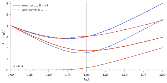
scripts/figures/tfim_spectrum.py) asserts agreement of each sector’s whole spectrum to at every dotted field. Levels at coincide.Figure 18.4 shows for three fields.
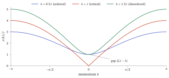
scripts/figures/tfim_dispersion.py.)18.6 What it buys
A complete solution: every eigenvalue and eigenvector of the chain, in both parity sectors (Theorem 18.6).
A conserved occupation for every mode, the data Lecture 19 needs to say what a relaxed state remembers.
The same free fermions elsewhere: at infinite repulsion Lecture 16’s gas has the free-fermion ground-state energy (Proposition 16.6), and Girardeau’s map makes it free fermions for every state, with a boundary condition that depends on (the reading at the end).
18.7 Caveats, in one place
Status. Theorem 18.3 and Theorem 18.6 are proved; the spectrum is also checked against exact diagonalisation at .
is even throughout; odd changes the bookkeeping of the grids and is not treated.
The two sectors are not optional. One boundary condition for both, or none, gives a quadratic model that is simple and wrong.
Free is special. Jordan–Wigner turns the Heisenberg chain’s term into a quartic one: its fermions interact, and it needed the Bethe ansatz.
18.8 Jordan–Wigner by hand, and local charges
Three sites by hand. On three sites, , , . Then , where and alone commuted. On states, the string at site sees the fermion at site or not, according to the order of creation.
The construction of local charges. Every occupation commutes with ; the local charges come from weighting whole blocks: for an even function , weight the term of in (18.13) by . The result commutes with block by block, and if the weighted coefficients are still trigonometric polynomials in , so the operator is a sum of fermion bilinears of range at most . The odd combinations also commute, because pairing creates and together and leaves alone. In spin language the first few are these.
Proposition 18.7 (Local charges of the TFIM sketched). Beside , the local charges commute with and with each other. is, in each sector, times the charge above, plus a constant. (The fermionic argument is the sketch; the commutators are checked exactly for .)
At and a computer search (the check script) finds that, modulo multiples of the identity, the conserved local charges of range at most three are spanned by , , , — at that size and coupling only. Spin forms follow from (18.7) and its analogues: a fermion bilinear on sites and carries the string of the sites between them, and on the ring the terms that wrap round pick up exactly as the boundary bond did, so one spin operator serves both sectors.
18.9 The quantum phase transition
Gaps.
From (18.14), (18.19) so the cheapest quasiparticle, at , costs : the quasiparticle gap. It closes at and nowhere else. The many-body gap — the distance from the ground state to the next level of the chain — is a different number, because each sector keeps only one parity of quasiparticle number. Riemann sums over the two grids are compared with one observation: for a -periodic function , over either grid vanishes unless divides , so (18.20) which tends to as for smooth , whose Fourier coefficients decay faster than any power.
Theorem 18.8 (Gaps of the TFIM). As through even values:
- (a)
if , the ground state is the even sector’s lowest state and the many-body gap tends to , the next level being the odd sector’s lowest, one quasiparticle at ;
- (b)
if , the lowest even and odd levels become degenerate, and the gap above this doublet tends to ;
- (c)
sketched the doublet’s splitting decays exponentially in , roughly like .
Proof. (a) For both signed energies (18.18) are positive and equal to , . The even sector’s excited states have at least two quasiparticles, so lie at least above . The odd sector’s lowest state has one quasiparticle, the cheapest, at : , so by (18.20); is smooth for . (b) For , , so the odd sector’s lowest state occupies and nothing else — odd, as required — and . Then by (18.20). Any other state of either sector differs from that sector’s lowest state in an even number, at least two, of occupations, each changing the energy by some ; so it lies at least above, and two quasiparticles at in the even sector come within of that bound. (c) extends analytically to complex up to its branch points, where or ; so decays like and (18.20) is dominated by .
For and the numbers are: doublet splitting , against a quasiparticle gap of , and the next level above the ground state, on its way to (check-l14-algebra.py). Each extra two sites cut the splitting by a factor approaching . At , the gap above the doublet is the two domain walls of §18.2.
Two phases.
The doublet is spontaneous symmetry breaking seen through a finite window. In the ordered phase the even and odd ground states are the finite- versions of ; their splitting is the amplitude to tunnel between the two ordered states, which needs a domain wall to sweep round the whole ring — hence exponentially small. As they become degenerate, and their combinations break the symmetry, with (the reading computes it). In the disordered phase the ground state is unique and gapped, and a quasiparticle is a dressed flipped spin.
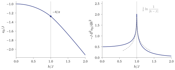
Between the phases the ground-state energy per site, (18.21) is continuous and has a continuous first derivative, but its second derivative diverges at , like (Figure 18.5) sketched: near and , , whose second -derivative integrates to a logarithm. A non-analyticity of the ground-state energy is what a quantum phase transition is, and the closing gap is its signature. At itself, and .
Duality.
Proposition 18.9 (Kramers–Wannier, on the spectrum). is symmetric under . Consequently the whole even-sector spectrum (18.16) at finite , and , are unchanged by ; the quasiparticle gap closes only at the self-dual point .
The operator form of the duality, and the XY chain, are in the next reading.
18.10 The XY chain, and duality as a map
The TFIM is one member of a family, (18.22) with anisotropy ; is the TFIM. (The literature writes for ; this course keeps for Lecture 16’s coupling.) The XY chain goes through the same three steps as the TFIM, with the same sectors and grids, and gives Theorem 18.6 with (18.23) and signed , unchanged (checked against exact diagonalisation at by the check script; the derivation is an exercise). The gap closes where both squares vanish: on the line , and on the segment , , where vanishes at (Figure 18.6). At the chain is the XX chain, which conserves the number of fermions; its momentum grids are compared below.
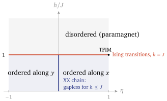
The XX chain () conserves the fermion number, and its -fermion eigenstates are Slater determinants of plane waves. As spin flips, hard-core bosons, two of them pick up only the exchange sign, , whatever their momenta, and Lecture 10’s periodicity condition becomes : exactly the NS or R grid of (18.10) for the sector of parity . The Heisenberg chain differs from the XX chain exactly in that its depends on the rapidities.
Duality. Behind this is an exact map of operators (Kramers and Wannier 1941, for the classical two-dimensional Ising model) cited: the domain-wall variables living on the bonds turn the bond term into a field and the field into a bond term, exchanging the ordered and disordered phases. It does not map the odd sector to itself — the signed mode changes sign — which is why the proposition says “even”. Kramers and Wannier’s use of it survives intact: if there is one transition, it must be at the self-dual point.
18.11 The conserved charges
The TFIM’s conserved charges are constructed directly, without a transfer matrix. Every occupation commutes with , but a single one is not local. Local combinations exist: weighting the term of in (18.13) by gives an operator that still commutes with , block by block, and whose coefficients are still trigonometric polynomials in — a sum of fermion bilinears of range at most . The first beyond is, in spins, (18.24) a local charge of range (the tutorial, and checked exactly for ). Continuing in gives about local charges, as for XXX in Lecture 15’s tower; Lecture 19 uses them to say which combinations of the a relaxed state remembers.
the linear action–angle system, : independent oscillators, each angle turning at a fixed frequency, and nothing scatters (§6.3)⟶free fermions, : independent modes, , two-body S-matrix whatever the momenta (type A, structural analogy: the same role, no limit taken)
18.12 Correlations as a Toeplitz determinant
Write and , so that , , and a bulk bond is by (18.7). Since , a product of fermion operators. In a Bogoliubov vacuum (a Gaussian state) such an expectation value is given by Wick’s theorem as a Pfaffian of two-point functions, and because and it collapses to a determinant (Lieb, Schultz and Mattis 1961) cited: in the thermodynamic limit (for finite the integral is the average over the NS grid). A matrix whose entries depend only on is a Toeplitz matrix, and the large- behaviour of Toeplitz determinants is a classical subject (Szegő’s theorem and its extensions). The results, due to Pfeuty (1970) and, for the XY chain, Barouch and McCoy (1971) cited: for the correlation tends to , so the spontaneous magnetisation is ; at it decays like ; for it decays exponentially. The check script confirms the determinant formula against exact diagonalisation at , and the ordered-phase limit at to six digits. Franchini’s Chapter 1 and its appendices carry this out in full.
18.13 The open chain and Majorana edge modes
Cut the ring: drop the boundary bond. There is then no parity-dependent term, no sectors, and one quadratic Hamiltonian on all of Fock space. Rewrite each fermion as two Hermitian Majorana operators, and , with and all different ones anticommuting. By (18.7) and , Each fermion is split in two, the field pairs the two halves on one site and the bond pairs halves on neighbouring sites. At the bonds pair with , and two Majoranas are left over, at the left end and at the right, appearing nowhere in . The fermion commutes with : it costs zero energy, every level is exactly doubly degenerate, and the two halves of this zero mode sit at opposite ends of the chain. In spin language these are, again, the two ferromagnets. For the zero mode survives with an energy exponentially small in (the check script measures ), localised near the ends; for it is gone. This is Kitaev’s chain (2001) cited, a model of a one-dimensional -wave superconductor: in the fermion language the ground-state doublet stays split only exponentially under sufficiently weak local perturbations that conserve fermion parity and do not close the bulk gap (a physical perturbation of fermions always conserves parity; the exact pairing of every level at is not what is protected), while in the spin language a weak longitudinal field , which is local for spins, splits it at once. The same algebra, read in two languages, gives a fragile symmetry breaking and a robust topological degeneracy (Franchini, §1.5).
18.14 Impenetrable bosons are free fermions
This lecture solved a chain by turning it into free fermions. Lecture 16’s interacting Bose gas, pushed to infinite repulsion, becomes free fermions — exactly, for every state and not only the ground state, by Girardeau’s map cited: Girardeau (1960). On a ring the map carries a boundary condition: taking one coordinate once round reverses its order with the other , so periodic bosons need fermions periodic for odd and antiperiodic for even . These are continuum fermions, ; this lecture’s live on a lattice with its own dispersion. What the two share is the structure, not the Hamiltonian.
Summary
- The model (18.1) and its parity , which splits the chain into an even and an odd sector.
- Jordan–Wigner (Theorem 18.3): spins become fermions through a string; the Hamiltonian is quadratic in each sector, with antiperiodic (even) or periodic (odd) boundary conditions.
- Fourier and Bogoliubov (Theorem 18.6): two grids of momenta, quasiparticles of energy , and every eigenvalue, sector by sector.
- Next: Lecture 19 quenches the chain and asks what it relaxes to.
References
P. Jordan and E. Wigner, Z. Phys. 47 (1928) 631 (the map); E. Lieb, T. Schultz and D. Mattis, Ann. Phys. 16 (1961) 407 (free fermions, the Toeplitz determinant); P. Pfeuty, Ann. Phys. 57 (1970) 79 (the TFIM solved); F. Franchini, An Introduction to Integrable Techniques for One-Dimensional Quantum Systems, Springer (2017), Chapter 1 (the XY chain, in full); G. B. Mbeng, A. Russomanno and G. E. Santoro, The quantum Ising chain for beginners, arXiv:2009.09208 (the two parity sectors, carefully); H. A. Kramers and G. H. Wannier, Phys. Rev. 60 (1941) 252; A. Yu. Kitaev, Phys.-Usp. 44 (2001) 131; M. Girardeau, J. Math. Phys. 1 (1960) 516.
End of Lecture 18
Free fermions: the transverse-field Ising chain
Lecture 18 · Contents
Keyboard
- → Space PgDn
- next screen, stopping before an equation, figure or statement it would cut
- ← PgUp
- previous screen
- ↓ ↑ wheel
- scroll freely
- Home End
- the start or the end
- S
- Full ↔ Spine, keeping your place
- T
- Think first on or off
- R
- reveal the next hidden proof
- C
- Core only on or off
- G
- contents: jump to a section or a statement
- + −
- text size
- D
- light or dark
- F
- full screen
- P
- pen on or off: draw on the text
- E
- erase the ink on the screen
- Z double-click
- enlarge an equation, figure or table; Z again for the next
- L
- laser pointer on or off
- B .
- blank the screen
- M
- move the toolbar: right, bottom, left, top
- ?
- this help
- Esc
- close a panel