19.1 The question

Lecture 0’s cradle did not thermalise, and Lecture 18 solved a chain with a conserved occupation for every mode. So the question is

if an isolated quantum system evolves unitarily, what relaxes, and to what?

The answer: local observables, when they relax at all, to the average in the ensemble fixed by a complete family of conserved charges (Definition 19.5); for the magnetisation after a field quench of the Ising chain this is proved (Theorem 19.7), and the Gibbs ensemble gets it wrong (Figure 19.2). The worked example is that quench.

19.2 Local and extensive charges

Densities

From here on the system is a ring of $N$ sites, each carrying a spin $\tfrac12$ : the Hilbert space is $(\C^{2})^{\otimes N}$ , site $N+1$ is site $1$ , and $\tau$ is the translation that moves every site one step, $n\mapsto n+1$ . An operator acts on a set of sites if it is the identity on every other factor.

Definition 19.1 (Local charge). A density of range $r$ is an operator $q$ acting on sites $1,\dots,r$ . On a ring of $N\ge r$ sites its local charge is the sum of its translates, $Q=\sum_{n=1}^{N}\tau^{\,n-1}(q),$ $\tau^{\,n-1}(q)$ acting on sites $n,\dots,n+r-1$ . The range $r$ and the density $q$ are fixed once and for all, and $N$ varies: a local charge is really one operator for each chain length. A local charge that commutes with $H$ is a local conserved charge.

The fixed range is the whole content: with $r=N$ allowed, any translation-invariant operator $A$ would qualify, as the sum of the translates of $A/N$ . The total spin $S^{z}=\sum_n S^{z}_n$ is a local charge of range $1$ , and so is a nearest-neighbour Hamiltonian such as Lecture 18’s Ising chain, of range $2$ . Local charges are extensive: $Q$ is a sum of $N$ terms of norm $\norm{q}$ , so $\norm{Q}\le N\norm{q}$ , and in a translation-invariant state $\langle Q\rangle=N\langle q\rangle$ — proportional to the length, as energy and particle number are. And local charges are rare.

Proposition 19.2 (Local charges are few). For each fixed $r$ , the local charges of range at most $r$ on a ring of $N\ge r$ sites form a vector space of dimension at most $4^{r}$ , whatever $N$ . So among the $2^{N}$ linearly independent conserved operators of a Hamiltonian with simple spectrum, the local conserved charges of range at most $r$ span at most $4^{r}$ dimensions.

Proof. A density of range $r$ is an operator on $(\C^{2})^{\otimes r}$ , a space of dimension $4^{r}$ , and $q\mapsto Q$ is linear. A density of smaller range is one of range $r$ that acts trivially on the last sites.

Two chains

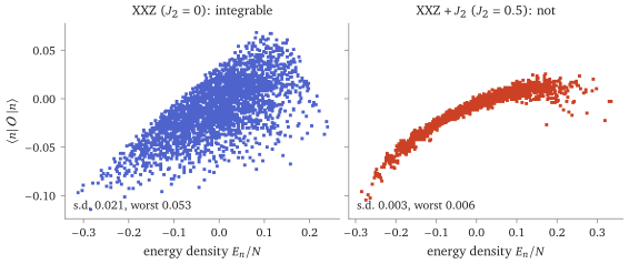
The chain is the XXZ chain with a next-nearest-neighbour coupling, $H=\sum_{n=1}^{N}\big(S^{x}_nS^{x}_{n+1}+S^{y}_nS^{y}_{n+1}+\XXZ\,S^{z}_nS^{z}_{n+1}\big) +J_2\sum_{n=1}^{N}\big(S^{x}_nS^{x}_{n+2}+S^{y}_nS^{y}_{n+2}+\XXZ\,S^{z}_nS^{z}_{n+2}\big).$ (19.1) At $J_2=0$ it is the XXZ chain, which the algebraic Bethe ansatz solves (Lecture 15’s reading); for $J_2\ne0$ it is not known to be integrable. Figure 19.1 compares $J_2=0$ with $J_2=0.5$ . The anisotropy is $\XXZ=0.55$ , away from the values $\cos(\pi p/q)$ with small $q$ at which XXZ acquires extra degeneracies.

19.3 Why integrable systems do not thermalise

Prepare a system in a pure state $\ket{\psi_0}$ that is not an eigenstate of $H$ and let it evolve. Nothing about $\ket{\psi(t)}$ relaxes: the state stays pure and, on a finite system, almost periodic. The question is about a local observable $\mathcal O$ (Definition 19.1), in the thermodynamic limit taken first. Expanding in eigenstates $H\ket n=E_n\ket n$ , $\bra{\psi(t)}\mathcal O\ket{\psi(t)} \;=\;\sum_{n}\abs{c_n}^{2}\bra n\mathcal O\ket n \;+\;\sum_{m\ne n}c_m^{*}c_n\,e^{-\ii(E_n-E_m)t}\bra m\mathcal O\ket n , \qquad c_n=\braket{n}{\psi_0} .$ (19.2)

Proposition 19.3 (Dephasing). On a finite system the time average of $\bra{\psi(t)}\mathcal O\ket{\psi(t)}$ over $[0,T]$ converges as $T\to\infty$ to $\tr(\rho_{\mathrm{d}}\mathcal O)$ , where $\rho_{\mathrm{d}}=\sum_EP_E\ket{\psi_0}\bra{\psi_0}P_E$ is the initial state dephased in energy and $P_E$ projects on the eigenspace of $E$ . If the spectrum is non-degenerate this is the diagonal ensemble $\sum_n\abs{c_n}^{2}\ket n\bra n$ .

Proof (★). The time average of $e^{-\ii(E_n-E_m)t}$ over $[0,T]$ is bounded in modulus by $2/(\abs{E_n-E_m}T)$ , so every term with $E_n\ne E_m$ tends to $0$ ; the terms with $E_n=E_m$ are exactly the ones the projectors keep, and the sum is finite.

So whatever a local observable settles down to is fixed by $\rho_{\mathrm{d}}$ — exponentially many numbers, and no ensemble worth the name. (Not by the $\abs{c_n}^{2}$ alone: inside a degenerate eigenspace the relative phases survive dephasing, and a spectator spin prepared in $\ket{{\pm}x}$ makes that visible.) Every relaxation statement is the claim that far fewer of those numbers matter.

The hypothesis that makes a generic system thermal

Definition 19.4 (Eigenstate thermalisation cited: Deutsch 1991, Srednicki 1994). A Hamiltonian satisfies the eigenstate thermalisation hypothesis (ETH) for a local observable $\mathcal O$ if, within each sector of fixed symmetry charges (such as $S^{z}$ and momentum) and in the bulk of its spectrum, $P_E\,\mathcal O\,P_E=\Big[\mathcal O_{\mathrm{mc}}(E/N) +\text{a fluctuation vanishing as }N\to\infty\Big]\,P_E ,$ (19.3) with $P_E$ the projector on energy $E$ within the sector and $\mathcal O_{\mathrm{mc}}$ a smooth function — the microcanonical average in that sector at that energy density. On a non-degenerate spectrum this is the familiar $\bra n\mathcal O\ket n=\mathcal O_{\mathrm{mc}}(E_n/N)+\dots$ ; where energies are degenerate it has to be asked of the whole block, or a spectator degree of freedom defeats it with every diagonal element right.

If (19.3) holds and $\ket{\psi_0}$ lies in one symmetry sector with subextensive energy fluctuations, Proposition 19.3 averages a smooth function over a narrow window and the answer is the microcanonical one: the system thermalises, in the only sense a closed quantum system allows. Nothing has been proved — ETH is a hypothesis about a Hamiltonian, checked numerically model by model, and (19.3), sector by sector, is exactly the statement a figure can test (Figure 19.1).

Figure 19.1. Eigenstate expectation values of the two-site operator

\mathcal O=S^{z}_1S^{z}_2

— equal, on the momentum eigenstates drawn, to the density

\tfrac1N\sum_nS^{z}_nS^{z}_{n+1}

, which is what is computed — in every state of one symmetry sector (

N=18

S^{z}=1

k=\pi/3

) of (19.1) at

\XXZ=0.55

: the two chains above, seen through an observable. Left, integrable, a cloud; right, with

J_2=0.5

, a curve. The two numbers say different things. Both are averages over windows of

32

consecutive states. The standard deviation in a window measures a typical eigenstate, and it falls in both models — for XXZ like

N^{-1/2}

(

\mathrm{sd}\sqrt N=0.091,0.091,0.090

N=14,16,18

). The largest deviation from a window’s median measures its worst eigenstate, and there they part: its average is

0.059,0.060,0.053

for XXZ, roughly flat, against

0.019,0.014,0.006

for

J_2=0.5

. Three sizes cannot settle a limit; they show the two chains differing as weak eigenstate thermalisation with persistent rare states would — and a quench does not sample eigenstates typically. The sector is fixed because in a degenerate subspace

\bra n\mathcal O\ket n

depends on the basis the diagonalisation happens to choose; in this sector neither the spin flip nor the reflection acts.

The charges are the memory

The left panel is not an accident of the observable. A chain with about $N$ local conserved charges, all commuting, can have its eigenstates labelled by all of them at once. What is expected to replace (19.3) there is a generalised eigenstate thermalisation: $\bra n\mathcal O\ket n$ a smooth function of the densities of a complete family of conserved charges — the strictly local ones for the Ising chain, quasi-local ones as well for the XXZ chain (Lecture 20’s reading) cited: Caux and Essler 2013. That reduces to a function of the energy alone only if the other densities are fixed by it, and they are not: two eigenstates at the same energy density generically carry different values of the other charges. The charges remember which state the system was prepared in, and a local observable can see the memory. The example this lecture proves is the Ising chain of Lecture 18, whose local charges are those of Proposition 19.8.

Free is linear

A quadratic Hamiltonian makes the Heisenberg equations linear: $\dd\gamma_k/\dd t=\ii\comm{H}{\gamma_k}=-\ii\varepsilon(k)\gamma_k$ , so each mode turns at its own frequency and ignores the others — the quantum form of the linear flow $\dot\varphi=\freq$ on a torus, and the reason there is no scattering.

(Lecture 18’s caveats say why this is special: the Heisenberg chain’s fermions interact.)

19.4 The generalised Gibbs ensemble, and a quench done in full

Definition 19.5 (Generalised Gibbs ensemble cited: Rigol, Dunjko, Yurovsky and Olshanii 2007). Given conserved charges $Q_a$ and their initial expectation values $\bra{\psi_0}Q_a\ket{\psi_0}$ , the generalised Gibbs ensemble is the maximum-entropy state reproducing all of them, $\rho_{\mathrm{GGE}}=\frac1Z\exp\Big(-\sum_a\beta_aQ_a\Big),$ (19.4) the multipliers $\beta_a$ being fixed by those expectation values.

With one charge, $Q_1=H$ , this is the Gibbs state and $\beta_1=1/T$ ; the question is what the others do. The claim to be tested — that a local observable relaxes to its $\rho_{\mathrm{GGE}}$ average — can be settled by calculation on Lecture 18’s chain.

The quench

Take the transverse-field Ising chain (18.1) at coupling $J$ , start in the ground state at field $h_0$ , and at $t=0$ change the field to $h$ . Both Hamiltonians are quadratic in the same fermions $c_k$ : only the Bogoliubov angle moves. Write $\theta_k$ for the post-quench angle of (18.15), $\theta^{0}_k$ for the pre-quench one, and $\chi_k=\theta_k-\theta^{0}_k ,\qquad \cos2\chi_k=\frac{a_ka^{0}_k+b_k^{2}}{\varepsilon_k\varepsilon^{0}_k},\qquad \sin2\chi_k=\frac{4J(h_0-h)\sin k}{\varepsilon_k\varepsilon^{0}_k} ,$ (19.5) with $a_k=2(h-J\cos k)$ , $b_k=2J\sin k$ , $\varepsilon_k=\sqrt{a_k^{2}+b_k^{2}}$ as in §18.5, and $a^{0}_k$ , $\varepsilon^{0}_k$ the same at $h_0$ . The rotation taking pre-quench modes to post-quench ones is the rotation by the difference angle, $\gamma_k=\cos\chi_k\,\gamma^{0}_k-\ii\sin\chi_k\,(\gamma^{0}_{-k})^{\dagger}$ , and the pre-quench ground state is the $\gamma^{0}$ vacuum.

Proposition 19.6 (The occupations are the conserved data). After the quench the post-quench mode occupations are $n_k=\bra{\psi(t)}\gamma_k^{\dagger}\gamma_k\ket{\psi(t)}=\sin^{2}\chi_k ,$ (19.6) independent of $t$ , and even in $k$ .

Proof. Each $\gamma_k^{\dagger}\gamma_k$ commutes with $H(h)$ , so its expectation is constant; its value in the $\gamma^{0}$ vacuum is $\abs{\sin\chi_k}^{2}$ by the rotation above. Evenness: $\cos2\chi_k$ in (19.5) depends on $k$ only through $\cos k$ .

The difference angle is not a bookkeeping convention: the sum angle gives a well-formed, plausible and wrong $n_k$ , off by as much as $0.48$ for $J=1$ , $h_0=0.4\to h=2.1$ .

What a local observable does

The transverse magnetisation $m^{z}=\tfrac1N\sum_n\sigma^{z}_n$ is the density of a one-site operator, and in a translation-invariant state it is $\langle\sigma^{z}_1\rangle$ exactly; (18.4) makes it $1-\tfrac2N\sum_kc_k^{\dagger}c_k$ .

Theorem 19.7 (Relaxation to the generalised Gibbs ensemble). Let $J,h,h_0>0$ with $h\ne J$ and $h_0\ne J$ . For the quench above on a ring of $N$ sites, with the NS momenta of the even sector, $m^{z}(t)=\frac1N\sum_{k}\Big[\cos2\theta_k\cos2\chi_k +\sin2\theta_k\sin2\chi_k\cos\big(2\varepsilon_kt\big)\Big] .$ (19.7) In the thermodynamic limit the sum becomes $\int\dd k/2\pi$ , the oscillating term tends to $0$ as $t\to\infty$ like $t^{-3/2}$ , and the limit is $m^{z}(\infty)=\int\frac{\dd k}{2\pi}\,\cos2\theta_k\,(1-2n_k) =\tr\big(\rho_{\mathrm{GGE}}\,m^{z}\big),$ (19.8) the average in the ensemble (19.4) built from the occupations (19.6).

Proof. The ground state at $h_0>0$ is in the even sector — in the $\sigma^{x}$ basis the field gives non-positive off-diagonal elements connecting every configuration, so Perron–Frobenius makes the ground vector unique and strictly positive, and $\Pi$ only permutes those configurations — so the NS grid is the right one. Each pair $(k,-k)$ then spans a two-dimensional even-parity space, and the expectation of $c_k^{\dagger}c_k$ in it is $\tfrac12(1-\cos2\theta_k\cos2\chi_k)-\tfrac12\sin2\theta_k\sin2\chi_k \cos2\varepsilon_kt$ ; summing gives (19.7). Every term is even in $k$ , since $\cos2\theta$ and $\cos2\chi$ are even and $\sin2\theta$ and $\sin2\chi$ are odd.

For the limit, $\varepsilon'(k)\propto\sin k$ vanishes exactly at $k=0$ and $k=\pi$ and nowhere else, and the amplitude is $\sin2\theta_k\sin2\chi_k =\frac{8J^{2}(h_0-h)\sin^{2}k}{\varepsilon_k^{2}\,\varepsilon^{0}_k} .$ (19.9) This is where the hypotheses are spent. With $h\ne J$ and $h_0\ne J$ neither $\varepsilon$ vanishes anywhere, so (19.9) has a double zero at both stationary points, and stationary phase with an amplitude vanishing to second order gives $t^{-3/2}$ — not the generic $t^{-1/2}$ of a non-vanishing amplitude. What is left is $\int\cos2\theta_k\cos2\chi_k$ , and $\cos2\chi_k=1-2n_k$ by (19.6). The ensemble (19.4) built from the charges $Q[f]$ below is diagonal in the occupations, so its modes are independent with occupations $n_k$ and the anomalous correlator $\langle\gamma_k^{\dagger}\gamma_{-k}^{\dagger}\rangle$ vanishes; the two numbers agree.

The hypotheses are spent there: at $h_0=J$ the zero of (19.9) is simple and the decay is $t^{-1}$ , at $h=0$ the dispersion is flat and nothing decays, and at $h_0=0$ there is no single ground state.

Figure 19.2. The quench

J=1

h_0=0.4\to h=1.9

. Left:

m^{z}(t)

from (19.7). In the thermodynamic limit (dark) it settles onto the generalised Gibbs value

0.4327

; the Gibbs value at the temperature

T=2.730

carrying the same energy is

0.5667

. At

N=32

(pale) nothing decays — the sum revives, and only its time average converges. Right: the conserved

n_k=\sin^{2}\chi_k

against the thermal occupations of the same energy; the closest Fermi–Dirac fit, at

T=3.24

, is out by

0.243

root mean square. The left panel’s formula is checked against exact diagonalisation of the spin chain at

N=8,10

, the initial state’s parity included.

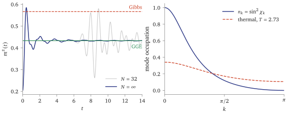
Theorem 19.7 takes $N\to\infty$ first and $t\to\infty$ second, and the two do not commute: at finite $N$ the sum (19.7) revives, as the pale curve of Figure 19.2 does, and only its time average converges.

Which combinations of the $n_k$ are local

Definition 19.5 asks for charges, and a single $n_k$ is not an observable of the chain: it is a sum over all $N$ sites whose coefficients never decay. Lecture 18’s reading built the local charges by weighting the $k$ -block of (18.13); this is that weighting.

Proposition 19.8 (The local charges of the Ising chain sketched). Let $J,h>0$ with $h\ne J$ , and let $f$ be an even function on the Brillouin zone. Write $Q[f]=\sum_kf(k)\big(n_k-\tfrac12\big)$ . Then $Q[f]$ is a sum of fermion bilinears whose real-space coefficients are the Fourier modes of $f\!\cos2\theta$ and $f\!\sin2\theta$ . Hence $Q[f]\ \text{has finite range}\iff f=\varepsilon\cdot(\text{a trigonometric polynomial}) ,$ (19.10) and $f=\varepsilon\cos mk$ gives a charge of range $m+2$ in the spins.

Proof sketch (★). In the pair basis $Q[f]=\sum_{0<k<\pi}\Psi_k^{\dagger}(f h_k/\varepsilon_k) \Psi_k$ , so the hopping and pairing functions are $A=fa_k/\varepsilon_k$ and $B=fb_k/\varepsilon_k$ . Finite range means both are trigonometric polynomials, and $a_k$ , $b_k$ are. For the converse, $g=f/\varepsilon$ is recovered from $A$ and $B$ by one identity, $(h+J\cos k)\,a_k-J\sin k\;b_k=2(h^{2}-J^{2}), \qquad\text{so}\qquad g=\frac{(h+J\cos k)A-J\sin k\,B}{2(h^{2}-J^{2})},$ (19.11) a trigonometric polynomial whenever $A$ and $B$ are — and this is exactly where $h\ne J$ is spent. Taking $f=\varepsilon$ returns $H$ itself; $f=\varepsilon\cos k$ returns $-\tfrac12Q_{+}$ of (18.24) up to a constant, checked against the even-sector ground state at $N=8,10$ , where the sign is visible.

The $\varepsilon$ weight is not decoration. Drop it, and $Q[\cos mk]$ is not local: its coefficients decay exponentially, at the rate $\abs{\ln(h/J)}$ — the branch points of $1/\varepsilon$ sit at $z=e^{\ii k}=h/J$ and $z=J/h$ , and whichever is nearer the unit circle sets the rate — without ever vanishing. Such a charge is quasi-local, the class that Lecture 20’s reading shows the XXZ chain needs. Both ends of the range are special: at $h=J$ the two branch points meet on the circle and the coefficients decay only like $1/d$ , while at $h=0$ , where $\varepsilon=2J$ is constant, the weight is a number and every trigonometric polynomial is strictly local again.

None of this weakens Theorem 19.7: knowing every $Q[\varepsilon P]$ is knowing every Fourier coefficient of $\varepsilon(k)n(k)$ , and $\varepsilon>0$ almost everywhere, so the strictly local charges fix $n_k$ almost everywhere and with it every local observable’s relaxed value. Numerically, keeping $Q[\varepsilon\cos mk]$ for $m\le M$ and maximising the entropy gives $m^{z}$ to $1.7\times10^{-3}$ at $M=4$ and $8\times10^{-8}$ at $M=16$ — and at $M=0$ , where only the energy is kept, that is the Gibbs ensemble, with exactly the error of Figure 19.2.

19.5 What it buys

Lecture 0’s question, answered in one model: after a quench the Ising chain’s magnetisation relaxes, and to the generalised Gibbs value, not the Gibbs one (Theorem 19.7, Figure 19.2).
Why: the occupations $n_k$ are conserved (Proposition 19.6), and the local charges fix them (Proposition 19.8); a local observable remembers them.
The ensemble that Lecture 20 carries to the interacting gas, where one function, the rapidity density, plays the part of the $n_k$ .

19.6 Caveats, in one place

Status. Proposition 19.3 (proof in a reading), Proposition 19.6 and Theorem 19.7 are proved; Proposition 19.8 is sketched. ETH is a hypothesis, checked numerically; generalised ETH is cited; the GGE’s definition is cited.
The hypotheses of Theorem 19.7 are spent. At $h_0=J$ the decay is slower, at $h=0$ it does not happen, at $h_0=0$ there is no single ground state, and at $h=J$ the observable $m^{z}$ cannot tell the Gibbs and generalised ensembles apart.
The order of the limits: $N\to\infty$ first, then $t\to\infty$ . At finite $N$ the magnetisation revives, and only its time average converges.
Which charges. For the Ising chain the strictly local charges fix the occupations almost everywhere (Proposition 19.8); for the XXZ chain the ultralocal charges are not enough, and quasi-local ones are needed (Lecture 20’s reading).
Every statement about a non-integrable chain is numerical, and a state that carries a thermal state’s charge densities relaxes to thermal values even in an integrable chain.

19.7 This was known in 1970

Remark 19.9 (This was known in 1970). Barouch, McCoy and Dresden computed the magnetisation of the XY chain after a field quench in 1970 and found it non-ergodic: it does not approach the equilibrium value. The ensemble that explains it was written down thirty-seven years later.

Summary

Local charges (Definition 19.1): fixed range, extensive, and few (Proposition 19.2).
Dephasing (Proposition 19.3): a local observable’s time average is fixed by the energy-dephased state (the diagonal ensemble when the spectrum is non-degenerate); ETH (Definition 19.4), sector by sector, makes it thermal in a generic chain.
The GGE (Definition 19.5): maximum entropy given all the charges.
The Ising quench (Proposition 19.6 and Theorem 19.7): the occupations are conserved, the magnetisation relaxes like $t^{-3/2}$ to the GGE value, and the Gibbs value at the same energy is different.
Next: Lecture 20 lets the ensemble vary slowly in space, and explains the cradle.

Worked in the tutorial: Exercise Sheet 19.

References

J. M. Deutsch, Phys. Rev. A 43 (1991) 2046, and M. Srednicki, Phys. Rev. E 50 (1994) 888 (eigenstate thermalisation); M. Rigol, V. Dunjko and M. Olshanii, Nature 452 (2008) 854; G. Biroli, C. Kollath and A. M. Läuchli, Phys. Rev. Lett. 105 (2010) 250401 (the rare states); M. Rigol, V. Dunjko, V. Yurovsky and M. Olshanii, Phys. Rev. Lett. 98 (2007) 050405 (the generalised Gibbs ensemble); E. Barouch, B. M. McCoy and M. Dresden, Phys. Rev. A 2 (1970) 1075; P. Calabrese, F. H. L. Essler and M. Fagotti, Phys. Rev. Lett. 106 (2011) 227203 (the Ising quench); F. H. L. Essler and M. Fagotti, J. Stat. Mech. (2016) 064002 (review); J.-S. Caux and F. H. L. Essler, Phys. Rev. Lett. 110 (2013) 257203; J.-S. Caux and J. Mossel, J. Stat. Mech. (2011) P02023 (counting charges).

The whole bibliography, lecture by lecture →