20.1 The question

Lecture 0 began with two clouds that passed through each other thousands of times and did not become one thermal hump. Lecture 17 gave the gas its equation of state, and Lecture 19 proved relaxation for a quench of the Ising chain; here the gas is assumed to be locally in a generalised Gibbs ensemble. So the question is

how does an integrable gas flow when its state varies in space, and what did the cradle show?

The answer: the density of each rapidity is carried at its dressed velocity ((20.5), (20.4)); for hard rods the dressed velocity is computed in one line (Proposition 20.1), and in the trap’s two free limits the flow is a rigid rotation that returns exactly (Figure 20.3). The worked example is hard rods.

20.2 Interacting models: one function carries the state

Free fermions made the argument exact, and easy, because the charges were quadratic. The replacement for an interacting model is already built: a macrostate in the thermodynamic limit is a root density $\rho(\bethe)$ , or the filling fraction $\vartheta=\rho/\rho_t$ of Definition 17.1, and every extensive charge is $\frac{\langle Q_a\rangle}{L}=\int q_a(\bethe)\,\rho(\bethe)\,\dd\bethe ,$ (20.1) with $q_a$ the charge’s one-particle eigenvalue — $q=k^{2}$ for the energy of the gas, $q=k$ for its momentum. A family of charges fixes $\rho$ exactly when its $q_a$ separate root densities; given such a complete family, the generalised Gibbs ensemble of Definition 19.5 is a single function — for a one-species gas; one filling per quasiparticle species in general, as the chain’s strings (Lecture 17’s reading) already needed — the same $\vartheta$ that Lecture 17 minimised the free energy over, now fixed by the initial state instead of by a temperature. Maximising (17.4) at fixed (20.1) is the generalised thermodynamic Bethe ansatz, and it returns (17.7) in dimensionless form: with $\eta=\ln(\rho_h/\rho)$ and $w=\sum_a\beta_aq_a$ , $\eta(\bethe)=w(\bethe)-\frac1{2\pi}\int K(\bethe-\mu) \ln\big(1+e^{-\eta(\mu)}\big)\,\dd\mu , \qquad \vartheta=\frac1{1+e^{\eta}}$ (20.2) cited. The multipliers carry the temperature, so (17.7)’s explicit $T$ ’s go: at thermal equilibrium $\eta=\varepsilon/T$ , and $w=(\varepsilon_0-\mu)/T$ returns Lecture 17’s equation exactly.

20.3 Generalised hydrodynamics

Now let the state vary in space: $\vartheta(\bethe,x,t)$ , slowly on the scale of the interactions — a local generalised Gibbs ensemble. That is the assumption, and the only one; there is no gradient expansion beyond leading order, which is what Euler scale means.

How fast does a quasiparticle actually move?

Lecture 12 found that a collision permutes the momenta and leaves a displacement behind (Theorem 12.2), and Lecture 11 found its quantum counterpart (11.7). A quasiparticle crossing a gas therefore collects one displacement per particle it passes, and does not travel at its bare velocity.

Figure 20.1. The effective velocity. Left: a tracer (dark) crossing a gas; each crossing displaces it, here forwards. Right: over many crossings the bare slope

\bethe

becomes an average slope

v^{\mathrm{eff}}

, which depends on the whole state through the rate at which crossings happen. For hard rods the bookkeeping closes in one line, (20.3); in general into Lecture 17’s dressing equation, (20.4).

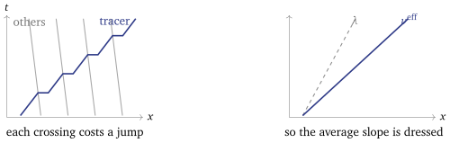
Proposition 20.1 (Hard rods sketched). Let the gas be $N$ identical rods of length $a$ and unit mass on a line, moving freely between elastic collisions, so that the bare momentum is $p_0(\bethe)=\bethe$ and the bare energy $\varepsilon_0(\bethe)=\bethe^{2}/2$ . Equal masses exchange velocities, so the set of velocities is only permuted and the gas is integrable; its rapidities are the velocities. A tracer of velocity $\bethe$ jumps forward by $a$ each time it passes a rod, so $v^{\mathrm{eff}}(\bethe)=\bethe+a\int\dd\alpha\,\rho(\alpha) \big[v^{\mathrm{eff}}(\bethe)-v^{\mathrm{eff}}(\alpha)\big] =\frac{\bethe-a\,\jmath}{1-a\,n} , \qquad n=\int\rho,\quad \jmath=\int\alpha\rho .$ (20.3)

Proof. The rate at which the tracer passes rods of velocity $\alpha$ is $\rho(\alpha)\abs{v^{\mathrm{eff}}(\bethe)-v^{\mathrm{eff}}(\alpha)}$ and the jump is $\pm a$ with the sign of the relative velocity, which is the first equality. Integrating it against $\rho$ gives $\int\rho v^{\mathrm{eff}}=\jmath$ identically, and substituting that back solves it.

Equation (20.3) is Equation (17.1) with the constant kernel $K=-a$ — not a local one: a delta-function kernel would dress every function by the same factor and cancel in the ratio. Dressing with it gives $2\pi\rho_t=(1)^{\mathrm{dr}}=1-an$ , the free volume fraction, and $(\varepsilon_0')^{\mathrm{dr}}=\bethe-a\jmath$ , whose ratio is (20.3). Lecture 17’s large- $c$ limit (the paragraph after Proposition 17.9) says this is no curiosity: to leading order in $1/c$ , and in the rest frame, the Lieb–Liniger gas is free fermions in a box lengthened by $2/c$ per particle, that is, a hard-rod gas of length $a=-2/c$ . In general $v^{\mathrm{eff}}(\bethe,x,t) =\frac{(\varepsilon_0')^{\mathrm{dr}}}{(k_0')^{\mathrm{dr}}} ,$ (20.4) with the dressing of (17.1) at the local $\vartheta$ and $k_0$ the excitation’s own bare momentum (Remark 17.3). Write it this way and not as $\varepsilon'/2\pi\rho_t$ , which is Equation (17.10). Lecture 17 got that by differentiating a thermal Yang–Yang equation driven by $\varepsilon_0-\mu$ ; differentiating (20.2) gives $\eta'=(w')^{\mathrm{dr}}$ instead, which dresses the combination $w$ and not the physical energy. (Free fermions with $w=\bethe^{4}$ : there $2\pi\rho_t=1$ and $\eta'=4\bethe^{3}$ , against $2\bethe$ from $\varepsilon_0=\bethe^{2}$ .) The two coincide at thermal equilibrium, where $\eta=\varepsilon/T$ and the $T$ cancels from the ratio — which is where Lecture 17 used it, saying explicitly that calling the ratio a propagation speed was not proved there. This section is where it is used, and the rods are the reason to believe it.

The equation

$\boxed{\ \partial_t\rho(\bethe,x,t) +\partial_x\big[v^{\mathrm{eff}}(\bethe,x,t)\,\rho(\bethe,x,t)\big]=0\ } \qquad\text{for every }\bethe .$ (20.5) One continuity equation per rapidity sketched: Castro-Alvaredo, Doyon and Yoshimura 2016; Bertini, Collura, De Nardis and Fagotti 2016: the number of quasiparticles of each rapidity is separately conserved — what integrability buys — and they are transported at the dressed velocity, which is what interaction costs. Ordinary hydrodynamics has five such equations in three dimensions; this has one per point of a continuum.

Figure 20.2. A lump of hard rods splitting, from (20.5): an excess of rods on a uniform background (palest) with rapidities near

\pm\bethe_0

separates into a left-mover and a right-mover — the Newton’s cradle with one collision instead of thousands. The rods have

a=1

and

an

reaches

0.40

, so the dressing is large: the dashed curve is the same initial state evolved with

a=0

, its peak

3.55

units behind. The circles are a direct simulation of the rods — no hydrodynamics — prepared as a genuine non-overlapping configuration and lying on the GHD curve to

3\%

of the lump height. The check script verifies that the solver conserves the number of rods to

10^{-12}

, separately in every rapidity slice.

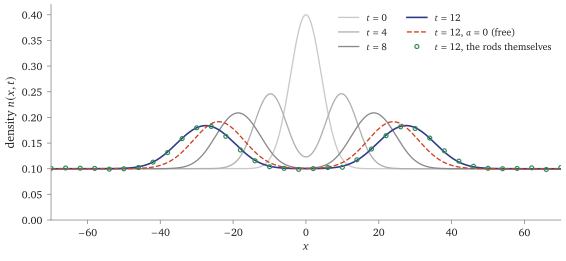
Figure 20.2 is the theory in one picture, and the one place in this course where an Euler-scale claim is tested against the microscopic model it describes: the circles are rods, evolved exactly, not a second solution of (20.5). The agreement is a law of large numbers and needs many particles per hydrodynamic cell — at one rod per ten units of length the same comparison fails outright.

20.4 The Newton’s cradle, finally

Figure 20.3. Lecture 0’s cradle (Figure 2), and what generalised hydrodynamics says about it. A harmonic trap adds the force term of (20.6). In the two free limits the characteristics are linear: the distribution turns rigidly in the scaled plane

(x,2\bethe/\omega)

at the trap frequency and returns to itself each period, so the clouds pass through each other and re-form, thousands of times. At intermediate coupling

v^{\mathrm{eff}}

depends on the local state, the turning is not rigid and the return is only approximate. The free skeleton of the mechanism, not a claim about every coupling.

Equation (20.5) has an equivalent form: the filling fraction is not conserved but advected, $\partial_t\vartheta+v^{\mathrm{eff}}\partial_x\vartheta=0$ in the homogeneous case — not obvious, since $v^{\mathrm{eff}}$ depends on $\vartheta$ cited: Castro-Alvaredo, Doyon and Yoshimura 2016. There a trapping potential $V(x)$ enters as a force on the rapidity, and the content is that quasiparticles follow characteristics: $\partial_t\vartheta+v^{\mathrm{eff}}\partial_x\vartheta -\partial_xV\,\partial_{\bethe}\vartheta=0 , \qquad\text{i.e.}\qquad \dot x=v^{\mathrm{eff}},\quad \dot{\bethe}=-\partial_xV ,$ (20.6) with $\vartheta$ constant along them cited: Doyon and Yoshimura 2017. In Lecture 11’s units, $\hbar=2m=1$ , the rapidity is the momentum: $\bethe$ obeys Newton’s second law and $x$ a dressed version of the first.

One caution first: (20.6) does not say the trapped model is integrable. A position-dependent potential breaks the homogeneous charges, no Bethe ansatz solves the trapped Lieb–Liniger Hamiltonian, and (20.6) is an Euler-scale approximation, good while $V$ varies slowly on the scale of the interactions cited: Doyon and Yoshimura 2017; Caux et al. 2019, App. H. It says two things.

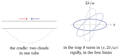
First, at the two ends of the coupling range the trap costs nothing at all. There $v^{\mathrm{eff}}=2\bethe$ — the ideal gas, and the impenetrable limit, where Girardeau’s map makes the gas free fermions in every state (Lecture 18’s reading) — and (20.6) is a linear flow of period $2\pi/\omega$ : the distribution turns rigidly on ellipses of fixed $x^{2}+(2\bethe/\omega)^{2}$ and returns exactly to itself (Figure 20.3). That is the cradle. In between, $v^{\mathrm{eff}}$ depends on the local state, the return is only approximate and the shape drifts — which is what the experiments see. Second, $\int\rho\,\dd x$ is in general not conserved in a trap, since (20.6) moves $\bethe$ : “the momentum distribution does not relax” means a shape returning, not a constant.

The theory, and then the data. Caux, Doyon, Dubail, Konik and Yoshimura applied GHD to the cradle geometry in 2019, at a coupling close to the original experiment’s. The first experimental test is Schemmer, Bouchoule, Doyon and Dubail’s atom chip: one cloud after a longitudinal trap quench, where GHD works and conventional hydrodynamics, which assumes local thermal equilibrium, does not. The quantitative test is Malvania, Zhang, Le, Dubail, Rigol and Weiss, in the same laboratory’s gases, measuring rapidity distributions directly through dozens of trap oscillations at $\gamma=c/n$ from $0.3$ to $9.3$ cited. There is, as of writing, no published comparison of generalised hydrodynamics with the 2006 data itself; theory and experiment meet in the later apparatus, not in the original plot.

What else spoils it. The atoms of Lecture 0’s tube are not exactly one-dimensional: virtually exciting a transverse mode and coming back leaves an effective three-body collision along the tube, which no Bethe ansatz solves, and whose rate sets a thermalisation time cited: Mazets, Schumm and Schmiedmayer 2008. Integrability is therefore approximate on two counts, and the question is one of time scales.

Remark 20.2 (Prethermalisation, and the quantum KAM question). Under weak integrability breaking a system started far from equilibrium first relaxes, on the fast scale, to the generalised ensemble of the unbroken model — a prethermal plateau — and only much later drifts to the thermal state, on a scale that grows as the breaking is reduced cited: Bertini, Essler, Groha and Robinson 2015; observed in Gring et al. 2012. This is the nearest quantum relative of Theorem 7.8, and the analogy is honest about where it stops: KAM is a theorem, with hypotheses, about which tori survive; prethermalisation is a statement about time scales with no theorem behind it. Whether approximate charges survive weak breaking in a controlled sense is the quantum KAM question, and it is open cited: Brandino, Caux and Konik 2015.

20.5 The map, closed

Lecture 0’s map named five ideas. Here is what each half of the course proved about them, and what it cited.

P1, integrability as a count. Part I proved it, with the statuses its lectures give: the Liouville–Arnold theorem (Theorem 5.7), action–angle variables (Theorem 6.5), and the Toda ring integrable (Theorem 9.10). In Part II the count is not a definition (Lecture 0’s caveat); a commuting family from one matrix takes its place.
P2, one family from one local identity. Proved on both sides: the quadratic bracket makes the Toda ring’s transfer matrices commute (Corollary 9.8), $RTT$ the Heisenberg chain’s (Theorem 14.3), and the quantum Toda chain proves that the second becomes the first as $\hbar\to0$ (Corollary 14.6).
P3, scattering that only rearranges momenta. The classical side cites Moser (Theorem 12.2); the quantum side derives the Yang–Baxter equation from three-body consistency (Theorem 13.3) and the Bethe equations from a ring: for the gas with a full proof that the Bethe wavefunctions are eigenstates (Lecture 11), and for the chain sketched in coordinates (Lecture 10) and proved algebraically (Lecture 15).
P4, densities, dressing and flow. Quantum only. The density equation is proved from an assumption (Lecture 16), the Yang–Yang equation from a count (Lecture 17), and the hydrodynamics of this lecture is sketched, with hard rods as its check.
P5, relaxation to a generalised ensemble. Proved for one quench and one observable of the Ising chain (Theorem 19.7); for the interacting gas it is the premise of this lecture’s hydrodynamics, and the cradle is only nearly integrable.

The dictionary between the two halves, typed: T a theorem of this course, an explicit proved map or $\hbar\to0$ limit between the columns; A a structural analogy, one role played by two separately established facts; C a citation. The column L is the lecture, or the optional lecture, where the Part II side lives.

Part I	Part II	L	type
Poisson bracket $\pb{\cdot}{\cdot}$	commutator $\comm{\cdot}{\cdot}/\ii\hbar$	14	A
$n$ integrals in involution	no agreed definition; criteria	0, A	A
Poincaré sections	level statistics	A	A
linear action–angle system	free fermions, $\sum\varepsilon(k)n_k$	18	A
$\oint p\cdot\dd q=2\pi\hbar n$	Bethe equations, logarithmic form	10	A
permuted momenta, braid	factorised S-matrix, Yang–Baxter	13	A
classical displacement	wave-packet displacement $\mp\theta'$	11	A
Lax matrix $L(\bethe)$	Lax operator $\Lop{n}(\bethe)$	14	T
Sklyanin bracket	$RTT$	14	T
$\rmat(\bethe)$	$\Rmat/\bethe=1+\ii\hbar\rmat+O(\hbar^{2})$	14	T
$\pb{\transfer(\bethe)}{\transfer(\mu)}=0$	$\comm{\transfer(\bethe)}{\transfer(\mu)}=0$	14	T
$\tr L^{k}$	$\dd^{k}\ln\transfer(\bethe)\|_0$	15	A
classical Yang–Baxter	Yang–Baxter	14	T
spectral curve $\det(z-\mono)$	T–Q relation	15	A, C
bands and gaps	Fermi sea of rapidities	16	A
frequency $\partial K/\partial I$	dressed velocity	17	A
measure $\dd I\,\dd\varphi$	Yang–Yang entropy	17	A
CM by reduction; isochrony	CS; equally spaced trapped spectrum	B	A
$\sllie_N$ roots	Dynkin-indexed nested equations	C	A, C
elastic non-diffractive scattering	labels transported by $X$	13, C	A
invariant tori	generalised Gibbs ensemble	19	A
KAM	prethermalisation	20	A, C

20.6 What it buys

One continuity equation per rapidity (20.5), with the dressed velocity (20.4) as the speed at which each rapidity is carried; hard rods show why (Proposition 20.1).
The cradle: in the two free limits the trapped distribution turns rigidly and returns exactly; between them it returns approximately.
The course closed: what each idea of Lecture 0’s map rests on, proved, sketched or cited.

20.7 Caveats, in one place

Status. Proposition 20.1 and (20.5) are sketched; the generalised thermodynamic Bethe ansatz, the advection form and the trap equation (20.6) are cited.
Euler scale. Generalised hydrodynamics is leading order in the gradients; the trap breaks the homogeneous charges, and the tube is not exactly one-dimensional, so the cradle is integrable only approximately.
No comparison with the 2006 data has been published; theory and experiment meet in later apparatus.
A complete family of charges is needed to fix the state, and for the XXZ chain the ultralocal ones are not enough (the reading).
Only the rows marked T are theorems, and all of them are Lecture 14’s.

20.8 When the ultralocal charges are not enough

The ultralocal charges are not enough. For the XXZ chain the charges generated by $\transfer(\bethe)$ as in Lecture 15 do not fix $\vartheta$ : two macrostates with different $\vartheta$ can share all of them, and quasi-local charges — the ones whose densities decay exponentially instead of stopping, exactly as $Q[\cos mk]$ did in Lecture 19 — are needed to close the ensemble cited: Ilievski, De Nardis, Wouters, Caux, Essler and Prosen 2015. This is where the free-fermion picture misleads if pushed: there the strictly local charges sufficed, because $\varepsilon$ never vanished.

20.9 More than one family

Remark 20.3 (More than one family). The labelled gases of optional lecture C carry two coupled families of rapidities, charge and spin. Nothing above changes in form: the macrostate is a pair $(\rho,\rho_{\text{spin}})$ , the charges are integrals against both, and the generalised ensemble is a pair of filling fractions coupled through the nested Bethe equations of optional lecture C. What changes is that the spin family carries no energy of its own ( $E=\sum k_j^{2}$ ), so the energy does not determine how the spin rapidities are distributed. It does not follow that the energy says nothing about them: the spin roots enter the charge equations and move the charge roots, so fixing the energy can exclude whole spin sectors — at $N=2$ , $L=c=1$ the zero-momentum singlet has $E=1.8439$ while every triplet state has $E\ge4\pi^{2}$ — and a thermal saddle couples the two families. What a generalised ensemble can do is be told a spin distribution that no temperature would have chosen.

Summary

One function carries the state: with a complete family of charges, the generalised Gibbs ensemble of a gas is a filling fraction $\vartheta$ , fixed by the generalised thermodynamic Bethe ansatz.
Hard rods (Proposition 20.1): a tracer jumps by $a$ at each rod, and $v^{\mathrm{eff}}=(\bethe-a\jmath)/(1-an)$ .
Generalised hydrodynamics (20.5): each rapidity’s density is carried at $v^{\mathrm{eff}}$ , the dressed velocity.
The cradle: in a trap the distribution turns and returns, exactly in the two free limits.
Beyond the path: optional lectures A (quantum chaos and level statistics), B (the Calogero–Moser systems) and C (nesting and the Hubbard model).

Worked in the tutorial: Exercise Sheet 20.

References

O. A. Castro-Alvaredo, B. Doyon and T. Yoshimura, Phys. Rev. X 6 (2016) 041065, and B. Bertini, M. Collura, J. De Nardis and M. Fagotti, Phys. Rev. Lett. 117 (2016) 207201 (generalised hydrodynamics); B. Doyon, SciPost Phys. Lect. Notes 18 (2020) (hard rods, Example 3.4; the external force, §4.5) and B. Doyon and T. Yoshimura, SciPost Phys. 2 (2017) 014; C. Boldrighini, R. L. Dobrushin and Yu. M. Sukhov, J. Stat. Phys. 31 (1983) 577 (hard rods); E. Ilievski et al., Phys. Rev. Lett. 115 (2015) 157201 (quasi-local charges); J.-S. Caux, B. Doyon, J. Dubail, R. Konik and T. Yoshimura, SciPost Phys. 6 (2019) 070 (the cradle geometry); M. Schemmer, I. Bouchoule, B. Doyon and J. Dubail, Phys. Rev. Lett. 122 (2019) 090601, and N. Malvania et al., Science 373 (2021) 1129 (the experiments); I. E. Mazets, T. Schumm and J. Schmiedmayer, Phys. Rev. Lett. 100 (2008) 210403; B. Bertini, F. H. L. Essler, S. Groha and N. J. Robinson, Phys. Rev. Lett. 115 (2015) 180601 (prethermalisation); G. P. Brandino, J.-S. Caux and R. M. Konik, Phys. Rev. X 5 (2015) 041043.

The whole bibliography, lecture by lecture →

Generalised hydrodynamics, and the quantum Newton’s cradle

What this lecture does