Lecture 8
Lax pairs, and the spectral parameter
Course map: G1, step 8 of 9. Lecture 5 said what integrals in involution buy, and nothing about how to find them. This lecture gives the method that finds them for the Toda chain: write the equations of motion as a matrix whose spectrum does not change. We prove that the spectrum is conserved, derive the Toda chain’s Lax matrix, close the chain into a ring, and rewrite the ring’s eigenvalue problem as a site matrix with a spectral parameter. We also say plainly what the method does not give: that the integrals commute. Lecture 9 proves that, from the site matrix.
8.1 The question: where do the integrals come from?
Definition 5.5 asks for independent first integrals in involution, and Theorem 5.7 turns them into tori. Neither says where the integrals come from. The ones we own came from two sources: the energy, and symmetry — angular momentum for a central force, momentum for a translation invariant system.
That is not enough for the models this course is built around. The open Toda chain of particles, (8.1) has two obvious integrals, and the total momentum , and no other evident continuous symmetry: apart from a common translation, no one-parameter family of transformations of the positions leaves invariant. In the early 1970s Ford’s numerical experiments on the periodic chain suggested that it was nevertheless integrable, and in 1974 Hénon and Flaschka independently proved it (Toda, §2.10). Flaschka’s construction, done here for the open chain, is the subject of §8.4. It works by finding a matrix , built from the ’s and ’s, whose eigenvalues do not move. eigenvalues, integrals.
So the question of this lecture is
where do the missing integrals of a many-body chain come from?
The answer is a Lax pair. We derive the Toda chain’s, close the chain into a ring, and rewrite the ring’s eigenvalue problem as a transport from site to site, with a spectral parameter (§8.7).
8.2 The Lax equation and isospectrality
Definition 8.1 (Lax pair). Let be a Hamiltonian on a phase space . A Lax pair for is a pair of smooth functions such that along every solution of Hamilton’s equations, and satisfy the Lax equation (8.2) is the Lax matrix; is its size, unrelated to .
The definition asks that Hamilton’s equations imply (8.2). In good cases the converse holds too, and (8.2) is the equations of motion, written as a matrix identity; we will see this for Toda, up to the motion of the centre of mass, which the Lax matrix cannot see.
Theorem 8.2 (Isospectrality). Let be a Lax pair for and a solution of Hamilton’s equations defined on an interval containing . Then:
- (i)
is constant in for every ;
- (ii)
, where solves , , and is invertible;
- (iii)
the characteristic polynomial is independent of : the eigenvalues of , with their multiplicities, are conserved.
Consequently each is a first integral, (Definition 2.3); if is complex, the real and imaginary parts of each are. If is antisymmetric, is orthogonal; if is anti-Hermitian, unitary.
Proof. (i) By the product rule and (8.2), and then because the trace is invariant under cyclic permutation, (The product rule gives terms ; cyclicity makes them equal.)
(ii) The equation is linear with coefficients continuous in , so its solution exists on the whole interval.1 Let solve , . Then , so and is invertible with . Now so .
(iii) .
Every point of lies on some solution, and (Definition 2.3), so (i) gives everywhere. Finally, if then , and the same line with the conjugate transpose gives the unitary case.
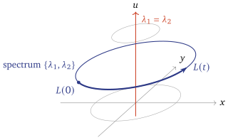
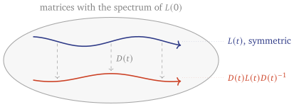
Part (ii) says more than (i): the flow moves inside one conjugacy class. For real symmetric and antisymmetric, is symmetric, so stays symmetric and moves by orthogonal conjugation (Figure 8.1).
For an matrix only of the can be independent: by the Cayley–Hamilton theorem is a combination of with coefficients that are polynomials in , so every with is a polynomial in the first . Equivalently, the conserved data is the characteristic polynomial, which has coefficients.
8.3 What a Lax pair does not give
Theorem 8.2 produces first integrals, and Definition 5.5 needs of them, independent and in involution. These are three different things. Having a Lax pair is no property at all: and form one for every . What matters is the spectral invariants a Lax pair delivers, and nothing in (8.2) makes them commute or makes enough of them independent. The Lax equation says how moves along one flow, the flow of ; involution is about the brackets of the with each other, which no single flow can see. For a particle in a central potential, and form a Lax pair, and by (5.3) and Leibniz Lecture 9 pays this debt for the Toda ring: it proves involution from a condition on the brackets of the entries of a Lax matrix, and checks independence.
8.4 The open Toda chain: Flaschka variables, and derived
unit masses on a line, positions , each repelled by its neighbours through the potential , which is large when particle has overtaken particle and small when they are far apart. With as in (8.1), Hamilton’s equations are (8.3) where the terms involving and are absent: the chain is open, and its end particles have one neighbour each. Lecture 0 met this potential. Here we find its Lax pair in two steps, after a change of variables that makes the equations polynomial.
Flaschka’s variables
The exponentials are the obstacle. Set (8.4) Then , and (8.3) becomes (8.5) with the convention — quadratic, with no exponential left. The map forgets one thing: shifting every by the same constant changes no . The centre of mass position is invisible to ; it is recovered from once the rest is known. Note also .
Step 1:
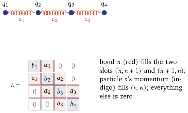
In the new variables a sum of squares, each counted twice. For a real symmetric matrix, is also a sum of squares, each off-diagonal entry counted twice because it appears as and . So the simplest with has each alone in a diagonal slot and each alone in a symmetric pair of off-diagonal slots. Which pair is a choice, and locality makes it: is the bond between particles and , so it goes in the slots and . The result is the symmetric tridiagonal (Jacobi) matrix of Figure 8.2; for , (8.6) Step 1 is a well-motivated choice, not a theorem; Step 2 is where it is tested.
Step 2: , from an ansatz
We want with , where is given by (8.5). Take antisymmetric, so that stays symmetric. is tridiagonal, and the commutator of two tridiagonal matrices has bandwidth at most two, so try the least that could work: antisymmetric and tridiagonal, with unknown functions. Compare the three bands of with those of .
Second off-diagonal. has none, but must vanish. So for every : with one common factor .
First off-diagonal. Only two terms survive: and (8.5) asks for . As this must hold for all , : , determined.
Diagonal. Nothing is left to choose, so this is the test: which is . It could have failed; it does not.
Proposition 8.3 (The Toda Lax pair). With the symmetric tridiagonal matrix with diagonal and off-diagonal , and the antisymmetric tridiagonal matrix with (8.7) the Toda equations (8.5) are equivalent to . Among antisymmetric matrices, is the only solution.
Proof. The three band computations above prove the Lax equation, and show that the tridiagonal ansatz has exactly this solution. The equivalence holds because the bands of are (8.5), entry by entry. For uniqueness among all antisymmetric matrices: if also works, is antisymmetric and commutes with . A Jacobi matrix with all has distinct eigenvalues: if , row gives from , row gives , and so on, so each eigenspace is at most one-dimensional. Diagonalise with orthogonal; then commutes with the diagonal of distinct entries, so it is diagonal, and it is antisymmetric, so it is zero.
So, to “where did come from?”: from and locality. And “where did come from?”: it was solved for, and it was the only possibility.
The integrals
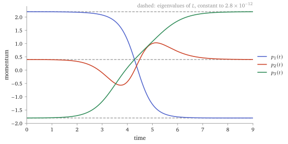
By Theorem 8.2, the functions , , are first integrals. The first three: (8.8) Total momentum, energy, and an integral cubic in the momenta. By Lecture 2’s one-line Noether theorem it too generates a symmetry of , but not a transformation of the positions alone, since its flow moves each at a rate that depends on the momenta. That is why nobody saw it. Figure 8.3 watches them at work for : the momenta change completely during a collision while the three eigenvalues of do not change at all. What the eigenvalues mean is Lecture 12’s business, and the figure already hints at it.
scripts/figures/toda_isospectral.py).8.5 Gauge freedom
A Lax pair is not unique, and the non-uniqueness has a structure worth knowing.
Proposition 8.4 (Gauge transformations). Let satisfy (8.2) along a solution, and let be invertible and differentiable in (for instance a function on phase space, evaluated along the solution). Then (8.9) satisfy , and has the same spectrum as .
Proof. With ,
Everything spectral is gauge invariant. Everything else is not: symmetry, the band structure, itself. For Toda, conjugate by with , . Then has on the diagonal, above it and below it: not symmetric, but with entries that are simpler functions of , and with the same characteristic polynomial. A reading at the end of the lecture draws the two as different paths on one isospectral set.
8.6 Periodic boundary conditions
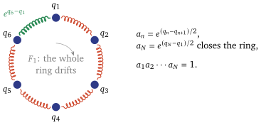
Put particles on a ring and let particle interact with particle across the join (Figure 8.4). With the positions read cyclically, , the Hamiltonian is (8.10) the open chain (8.1) with one more spring, . The equations of motion are those of the open chain with every index read modulo : , . For , in centre-of-mass coordinates and after a rescaling, this is the Hamiltonian (7.7) whose Poincaré section Figure 7.5 showed smooth curves where Hénon–Heiles had chaos. Lecture 9 proves that what the figure showed is integrability.
The Lax pair of the ring
Flaschka’s variables (8.4) carry over with one more bond, , and one new constraint: the exponents telescope to zero round the ring, so (8.11) Put in the two corners: (8.12) Let be antisymmetric with for every , indices modulo , so that . The band computations of Proposition 8.3 go through with the indices read modulo (for the second-neighbour terms, which cancel identically, land on first-neighbour slots and change nothing), so for , and by Theorem 8.2 the are conserved, with and .
8.7 The site matrix
The eigenvalue problem of the ring’s Lax matrix is a recursion, (8.13) closed up by and . The recursion (8.13) is of second order, so it is a first-order recursion for pairs . Solving for means dividing by , which gives a matrix of determinant involving two bonds. A gauge transformation does better.
The gauge that makes it local
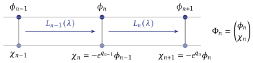
Conjugate by , the gauge of Proposition 8.4 (it is §8.5’s up to a constant). In the new variable , (8.13) reads (8.14) the coefficient of is now . (Substitute in (8.13), use , and divide by .) Now collect a pair, . Then (8.14) and the definition of the second component say exactly (8.15) This is the site matrix: local (site only), polynomial in the spectral parameter , and a transport one step along the lattice (Figure 8.5).
8.8 What it buys
integrals for the Toda ring, the for , from one matrix whose spectrum does not move. Energy and total momentum are two of them; the rest were invisible as symmetries of the positions.
A site matrix with a spectral parameter. The ring’s eigenvalue problem is a product of matrices (8.15), each built from one site’s alone. Lecture 9 multiplies them round the ring and proves, from one identity that a single site matrix satisfies, that the integrals commute.
A method: choose from and locality, then solve for .
8.9 Caveats, in one place
Status. Theorem 8.2, Proposition 8.3 and Proposition 8.4 are proved. The ring’s Lax pair is the band computation of Proposition 8.3 with indices read modulo , and the site matrix (8.15) is derived.
Conserved is not in involution (§8.3); Lecture 9 proves involution, and independence, for the ring.
The ring still drifts. The flow of , , changes no , so no level set is compact; Lecture 9 splits the drift off.
is degenerate. The corner slot is the off-diagonal slot, so and . The formulas here are for .
8.10 The Euler top: a Lax pair whose spectrum misses an integral
A rigid body turning freely about its centre of mass, described in the body frame, the principal axes of inertia moving with the body. The principal moments are ; the angular momentum and the angular velocity have body components and , with . In space is constant; the body frame turns with angular velocity , so , which are Euler’s equations (8.16) in components and cyclically. We use them only as a differential equation on . (These are moments of inertia, not the integrals of Theorem 8.2 nor Lecture 6’s actions; the standard names are kept.) (The phase space of the body is , of dimension ; the three components of are functions on it, and (8.16) is the part of the motion that does not involve the orientation.)
The Lax form
For let be the antisymmetric matrix with : Then : apply both sides to and use the Jacobi identity of the cross product, . Hence, with and , Euler’s equations are (8.17) a Lax equation with . The student already knew it; only the notation is new.
What does it conserve? is real antisymmetric, so and ; indeed (8.18) The spectrum knows and nothing else. But the energy is also conserved, since , and unless it is not a function of . This is the insufficiency discussed in §8.3: a genuine Lax pair, for a genuinely integrable system, whose spectrum misses the second integral. §8.11 gets it back.
The motion, from the two integrals
Take . Both integrals together confine to the intersection of the sphere with the ellipsoid (Figure 8.6). On the sphere is smallest at and largest at , and near these four points the level curves are small closed loops. The equilibria of (8.16), where , are the six points : steady rotation about a principal axis. The middle level, , is (8.19) two planes through the axis, cutting the sphere in two great circles that cross at : the separatrix.
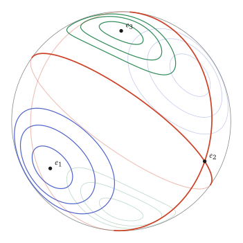
scripts/figures/euler_sphere.py, which checks that and are conserved along each). The separatrix (red) is drawn from (8.19): two great circles, made of the equilibria and four orbits running between them. The far hemisphere is faint.Theorem 8.5 (The tennis-racket theorem). Let and . Steady rotation about the axis of smallest or of largest moment is stable: for every there is such that implies for all , and the same for . Steady rotation about the middle axis is unstable: there are solutions starting arbitrarily close to that tend to .
At the board the proof is Figure 8.6: near and the conserved quantities confine to small loops, while every neighbourhood of meets the separatrix, which runs to the opposite pole. The reading turns both halves into estimates.
Proof. Stability at . The function is conserved and vanishes at . So for all , and is small when is near . Since is conserved, stays close to ; cannot pass through , so it keeps its sign and stays close to . At use instead.
Instability at . The components of are , and ; with distinct moments they all vanish only when two components of do, so the equilibria are the points . Each open arc of the separatrix between and contains no equilibrium, so a solution started on it moves along it with nowhere-vanishing speed, so monotonically; being bounded, it converges as , and the limits can only be equilibria. So each arc runs from one end to the other. It remains to see that some arc leaves . The map combined with takes solutions of (8.16) to solutions (check it on the three components, each of which is a product of the other two ’s), fixes , exchanges the two planes of (8.19) and reverses time. So if the arc in one plane runs into , its mirror image runs out of it, towards . Its points can be taken as close to as we like.
Throw a tennis racket or a phone spinning about its middle axis: it flips, and off the separatrix it flips back periodically, because a nearby orbit follows a loop that runs close to the separatrix, round to near and back (Figure 8.7).
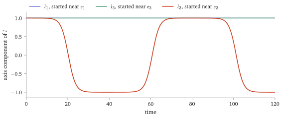
scripts/figures/tennis_racket.py, which asserts both).Poinsot’s construction
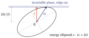
The same two integrals give Poinsot’s picture of the motion in space. In the body, the angular velocity lies on the energy ellipsoid , since . The normal to at is the gradient , and the tangent plane there lies at distance from the centre. In space is a fixed vector and a fixed number, so this tangent plane is the same plane at all times, the invariable plane. The point of contact is , which lies on the instantaneous axis of rotation and so has zero velocity. Hence:
Proposition 8.6 (Poinsot). The energy ellipsoid, carried by the body, rolls without slipping on a fixed plane perpendicular to at distance from the centre.
Remark 8.7 (The other tops). The symmetric heavy top of Lagrange and the Kowalevski top also have Lax pairs, both with a spectral parameter of the kind §8.11 introduces cited: Audin, Spinning Tops, ch. II §2 and ch. III §2. We do not use them.
8.11 Gauge, and a spectral parameter
The warning to carry forward: the Poisson brackets of the entries of , which Lecture 9 will make the key to involution, change under a gauge transformation even though the spectrum does not. And the site-matrix section of this lecture uses a gauge transformation to make the periodic chain’s Lax representation local, built site by site; Lecture 9 uses the resulting site matrices to prove involution.
The Euler top left a problem: for a body whose moments are not all equal, its Lax matrix conserves and misses (the insufficiency discussed in §8.3). Manakov’s repair (1976) is to let the Lax matrix depend on an extra complex number , the spectral parameter.
Put with , so that and cyclically. Since , this gives . Now set (8.20) Then for every : the term is (8.17), the term is , and the term is , which vanishes because .
So Theorem 8.2 applies at each separately, and the characteristic polynomial of is conserved as a polynomial in two variables. It is (8.21) where the first term involves only the constants , and The coefficient of contains : the integral that missed is a spectral invariant of . (For a spherical body is a multiple of , only shifts the spectrum, and there was nothing to recover.) All three identities are checked symbolically in scripts/check-l7-algebra.py.
This is the first thing a spectral parameter is for: one matrix family carries more invariants than one matrix, since every coefficient of every power of in is conserved. There are two more, and they are the reason Part I keeps from here on.
A curve. The conserved polynomial defines the spectral curve , which the flow leaves unchanged; its coefficients are the integrals. For the Toda ring, Lecture 9’s reading forms a different but related curve, from the monodromy , identifies its finite gaps from , and cites their relation to the action variables. (Here is local notation.)
A bracket. For the Toda ring, Lecture 9 checks a bracket that compares the site matrices and at two different values of the parameter, composes it for their product round the ring, and proves that the traces at and commute. That pays this lecture’s IOU for the ring. Manakov’s matrix is a separate example of what a spectral parameter can encode.
8.12 Time evolution, zero curvature and plaquette holonomy
Time evolution, and zero curvature
The site matrix transports in space. Transport in time is a second matrix at each site, (8.22) which follows from , the recursion and the same gauge (we omit that derivation; what matters is the next statement, checked directly).
Proposition 8.8 (Discrete zero curvature). For every , (8.23) holds if and only if and : the equations of motion of the ring.
Proof. Multiply out: Every has cancelled on the right. The off-diagonal entries agree iff , the diagonal ones iff has the stated value.
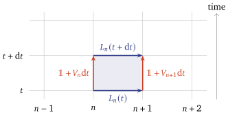
Why “curvature”? Draw the lattice of sites and times (Figure 8.10). Put on each horizontal link, as transport from site to , and on each vertical link, as transport from to . Go round one plaquette, out along one pair of sides and back along the other: (8.24) This is the holonomy of the plaquette. In a flat geometry transport is path-independent and every small loop has trivial holonomy; so (8.23) says the connection on the space-time lattice is flat. It is the discrete form of the zero-curvature condition (8.25) to which (8.23) reduces if , and terms of order are dropped. That equation, which integrates KdV and sine-Gordon, belongs to the sequel on field theory; it appears here once. The site-by-site transport, and its product round the ring, is the architecture Lecture 14 quantises, with the Sklyanin bracket becoming the relation.
Summary
- Lax pair (Definition 8.1): along the flow. Then the spectrum of is conserved and the are first integrals (Theorem 8.2); only of them are independent.
- Conserved is not in involution: nothing in the Lax equation makes the commute (§8.3).
- Toda: in Flaschka’s variables is the symmetric tridiagonal matrix fixed by and locality, and is solved for and unique (Proposition 8.3); the first integrals are (8.8).
- The ring: in the corners and ; the are conserved for .
- The site matrix: in a gauge that makes it local, the eigenvalue problem is the transport , with (8.15).
- Next: Lecture 9 multiplies the site matrices round the ring and proves that the integrals commute.
References
Babelon, Bernard and Talon, Introduction to Classical Integrable Systems, ch. 3 (Lax pairs) and ch. 2 on Toda; Toda, Theory of Nonlinear Lattices, §§2.10–2.11 (Flaschka’s variables and the periodic chain); H. Flaschka, Phys. Rev. B 9 (1974) 1924; M. Hénon, Phys. Rev. B 9 (1974) 1921; M. Audin, Spinning Tops (the Euler top, in the reading).
A linear equation cannot blow up in finite time: Grönwall’s inequality bounds by . This is the only fact about ODEs used beyond Theorem 1.5.↩︎
End of Lecture 8
Lax pairs, and the spectral parameter
Lecture 8 · Contents
Keyboard
- → Space PgDn
- next screen, stopping before an equation, figure or statement it would cut
- ← PgUp
- previous screen
- ↓ ↑ wheel
- scroll freely
- Home End
- the start or the end
- S
- Full ↔ Spine, keeping your place
- T
- Think first on or off
- R
- reveal the next hidden proof
- C
- Core only on or off
- G
- contents: jump to a section or a statement
- + −
- text size
- D
- light or dark
- F
- full screen
- P
- pen on or off: draw on the text
- E
- erase the ink on the screen
- Z double-click
- enlarge an equation, figure or table; Z again for the next
- L
- laser pointer on or off
- B .
- blank the screen
- M
- move the toolbar: right, bottom, left, top
- ?
- this help
- Esc
- close a panel