Lecture 9
Why the integrals commute: the Toda ring is integrable
Course map: the last step of G1, and the classical half of G5. Lecture 8 found the conserved quantities of the Toda ring — the spectrum of its Lax matrix — and left a debt: conserved is not the same as in involution, and Definition 5.5 asks for both. This lecture pays the debt. It packages all integrals into one function of a spectral parameter, the transfer matrix, proves that its values Poisson-commute from a single identity satisfied by a single site, checks independence, and applies Theorem 5.7: the periodic Toda chain is Liouville integrable, and its motion winds round tori that drift. The identity is the one Lecture 14 quantises.
9.1 The question
The Toda ring of Lecture 8 has particles on a circle, (9.1) and its Lax matrix has a spectrum that does not change in time (Theorem 8.2), so the numbers are conserved. Lecture 8 also rewrote the eigenvalue problem of as a transport from site to site, , with the site matrix (9.2) which contains the variables of site and nothing else.
Definition 5.5 asks for more than conservation: integrals that Poisson-commute with each other and are independent. Nothing in the Lax equation says anything about brackets between the . So the question of this lecture is
are the Toda ring’s integrals in involution and independent — and if so, what does its motion look like?
The plan has three steps. Build all the integrals at once, as the coefficients of one polynomial (§9.2). Show that follows from one identity satisfied by one site matrix (§§9.3 to 9.5). Then independence and Theorem 5.7 do the rest (§§9.6 and 9.7).
9.2 All the integrals at once: the transfer matrix
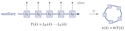
Transport all the way round the ring.
Definition 9.1 (Monodromy and transfer matrices). For a chain of sites with site matrices , the monodromy matrix and the transfer matrix are (9.3) The chain is ultralocal if variables at different sites Poisson-commute: for . When tensor legs are also in play (§9.3), the site moves to a superscript: .
The Toda ring is ultralocal, since involves only . By (9.2), , and is what a solution of the recursion picks up in one circuit (Figure 9.1).
What the transfer matrix contains
Expand the product (9.3) as a sum over paths through the index values of the factors. The entry forbids a path to stay at , so each visit to enters through and leaves at the next site through : a factor in place of two factors . The trace closes the path, so the pair may straddle the join. Hence (9.4) the sum over sets of bonds, no two sharing a site, with the sites they cover. Writing , (9.5) So is a polynomial of degree whose non-trivial coefficients are functions on phase space, and is one of their functions.
The same integrals as Lecture 8’s
A number is an eigenvalue of Lecture 8’s Lax matrix exactly when its eigenvalue recursion has a solution with . The gauge that turned the recursion into respects periodicity, since , so this happens exactly when has an eigenvalue : when , using . For , and are both monic of degree . Where the spectrum of is simple they have the same roots, so they are equal there. Such points are dense: at fixed , momenta far enough apart make the discs of Gershgorin’s theorem disjoint and the spectrum simple, so the discriminant of is a non-zero polynomial in , and its non-zero set is dense. Both sides are continuous in , so sketched (9.6) The are therefore, up to sign and the constant , the elementary symmetric functions of the eigenvalues of . Newton’s identities turn them into the and back. They are Lecture 8’s integrals, reorganised, and they are the candidates for Definition 5.5. Everything now turns on their brackets.
9.3 The notation the proof needs: tensor legs
is a matrix whose entries are functions on phase space. What we need is the collection of all their brackets, , sixteen functions at once. The trick is to package them as a single matrix acting on , with .
Definition 9.2 (Tensor legs). Write for the matrix unit with a in row , column , and recall . For matrices , put , , and (9.7)
The subscript is a leg, not a matrix index: is the whole matrix , placed in the first factor (Figure 9.2). The right-hand form of (9.7) is the one to memorise: the entry in row and column is the bracket of the entry with the entry.

Remark 9.3 (Two brackets in one formula). and commute as matrices, , because they act in different factors. Their entries do not Poisson-commute: that is what (9.7) records. The composition theorem below turns on the first fact at its decisive step; nothing uses , which is false.
One matrix on appears everywhere below.
Definition 9.4 (Permutation operator). ; equivalently .
Proposition 9.5 (Properties of ). ; , so commutes with every ; and (9.8)
Proof. swaps twice. For (9.8), expand and use : the sum collapses at , . The middle property follows by applying both sides to .
9.4 One identity for one site: the quadratic Sklyanin bracket
Here is the structural assumption that will force involution. It is a statement about the brackets of one site matrix at two values of the spectral parameter, and it involves one fixed numerical matrix.
Definition 9.6 (Quadratic Sklyanin bracket). A site matrix satisfies the quadratic Sklyanin bracket with classical -matrix , a matrix of numbers, if (9.9)
The left-hand side is sixteen unknown brackets. The right-hand side says they are all determined by the matrices themselves and one numerical , which is slid past the product from both sides (Figure 9.3). Why this form and not another is the content of the next theorem: it is the form that survives multiplication.

Theorem 9.7 (The quadratic bracket composes). If the chain is ultralocal and every site matrix satisfies (9.9) with the same , then so does the monodromy matrix: .
Proof. Take ; the general case is the same telescoping. Leibniz and ultralocality kill the cross terms, and matrices in different legs commute (Remark 9.3), so with and , the two sites’ pairs, and , again because leg- and leg- matrices commute.
Corollary 9.8 (Commuting transfer matrices). for all . Hence the coefficients of are in involution.
Proof. Take the trace over both factors, : , because the trace of a commutator vanishes. Expanding in and , every coefficient Poisson-commutes with every other. At the identity follows by continuity.
So the whole question of involution has been reduced to one identity for one matrix. That is where the work of this lecture is.
9.5 The worked example: the Toda site matrix
Proof. Only involves , so the only non-zero brackets pair it with an off-diagonal entry. With , and , both independent of and . By (9.7), with ; the last step is (9.8) applied to each term. On the right of (9.9), write . The permutation commutes with every (Proposition 9.5), which removes the and the terms, and it turns into , so Dividing by gives the left-hand side. The chain is ultralocal, so Theorem 9.7 lifts the identity to , and Corollary 9.8 gives the involution.
Read the first displayed line as the tensor-leg drill: it is the sixteen brackets of (9.2), of which four are non-zero, written as one matrix. If that line is not comfortable, nothing after it will be. As an exercise, find the four non-zero brackets and assemble the matrix.
9.6 The theorem
Theorem 9.10 (The periodic Toda chain is Liouville integrable). On the coefficients of are in involution and independent on a dense open set, and . The periodic Toda chain satisfies Definition 5.5.
9.7 The proofs
Proof of Theorem 9.10. Involution is Proposition 9.9, and (9.5) is . So : every is conserved. Conservation comes out of involution and needs no separate argument.
Independence. Read (9.4): , where is the -th elementary symmetric polynomial of the momenta and every term of has a factor and degree at most in (each bond removes two factors ). In the Jacobian the part of top degree in therefore comes from the alone, and it is , the Vandermonde determinant. So at fixed the Jacobian is a non-zero polynomial in , which cannot vanish on any open set. Where it does not vanish the are independent; that set is open, and it meets every open set, so it is dense.
The proof of the second theorem has four steps, and only the first two use the Toda chain at all. Write for the springs.
Proof of Theorem 9.11. (i) Bounded. Every term of is positive. On the value is fixed, since is a function of and , so and for every . The springs’ exponents telescope to zero round the ring, so , and each . (By the inequality of arithmetic and geometric means , so these bounds are not vacuous.) Every gap therefore lies in . Each is a fixed linear combination of the gaps, so at fixed every is bounded too. The slice is closed and bounded: compact.
(ii) Complete. Let for constants . By involution is constant along the flow of , so the bounds of (i) hold along every integral curve. The components of are polynomials in the and the , hence bounded by a constant on the curve, which in a time moves at most a distance and so stays in a compact ball. By the escape argument of Proposition 1.7, a curve that exists only up to a finite time must leave every compact set. So every such flow is complete.
(iii) Cylinder. Stages (i)–(iii) of the proof of Theorem 5.7 and the first half of stage (iv) (§5.5) use involution, independence on , connectedness and complete flows, and nothing else. They make the orbit of an action of with a discrete stabiliser , so (Lemma 5.10).
(iv) Drift. Shifting every by is the same as shifting by in (9.4), so is a constant multiple of , constant on . Hence changes at a constant rate along each flow, and at the time- point is for a linear map , not zero since . A period does not move , so , and . That is compact by (i), so is a lattice of full rank in (Lemma 5.10): the slice is and . Stage (vi) of the proof of Theorem 5.7 makes the flow of linear.
Step (i) is the only place the ring matters. On the open chain nothing ties the springs together, a single spring can be made as weak as one likes at fixed energy, and the level sets stay unbounded even after the drift is removed: the open chain scatters instead of winding.
9.8 What it buys
The motion. On every regular level set the flow of is a straight line in coordinates on : it winds round the torus while the centre of mass moves along at the constant speed , possibly zero. For , with the centre of mass removed, the tori meet the Poincaré section of Figure 7.5 in its closed curves: the numerical plot of Lecture 7, beside the chaos of Hénon–Heiles at the same energy, illustrates this theorem at .
Action–angle variables need one more step. Separate the centre of mass canonically, fix the total momentum, and relative degrees of freedom remain, whose regular level sets are the compact tori of Theorem 9.11. To those Theorem 6.5 applies. As an exercise, carry out the separation for with , , and ; the two-particle ring at the end of the readings does it. Computing the actions needs the curve of the reading below, with one action for each of its gaps cited: Flaschka and McLaughlin 1976.
The method. Three moves did everything, and none of them is special to Toda:
one identity, (9.9), for one site matrix;
composition along the chain, Theorem 9.7, which needs only ultralocality;
the trace, which kills a commutator.
Change the site matrix and the -matrix, and the same three moves give commuting integrals for another chain. Lecture 14 replaces the Poisson bracket by the commutator and by an -matrix with . The same three moves then give the commuting transfer matrices of the Heisenberg spin chain, and on the quantum Toda chain their limit is exactly (9.9) with (9.10). That is goal G5, and the one row of the classical-to-quantum dictionary that is a theorem rather than an analogy.
9.9 Caveats, in one place
Three things a careful reader should know, collected here so that the arguments above can run without interruption. (The linear bracket, which this lecture does not need, is in the reading.)
Independence is generic, not universal. Theorem 9.10 proves independence on a dense open set, and that is all Definition 5.5 asks. It does fail somewhere: at the equilibrium , every flow is a drift.
The ring drifts. The flow of translates every and changes no spring, so no level set is compact. Tori appear only after the centre of mass is fixed, which is why Theorem 9.11 is stated for slices.
The sign of belongs to the site matrix. Other books use the site matrix with exchanged, which gives ; mixing a sign with the wrong site matrix breaks (9.9).
9.10 The same integrals from zero curvature, and the route not taken
Conservation directly. (Lecture 8’s reading has the fuller version, with the plaquette picture.) Involution gave conservation for free, but is also conserved for a more geometric reason. With , the equations of motion of the ring are equivalent to for every and every : transport in space and in time commute round every plaquette of the space-time lattice, a discrete zero-curvature condition. Differentiating the product (9.3), the sum telescopes to , a Lax equation for the matrix , and is conserved. Periodicity is used once, to identify with .
The route not taken. One can prove integrability of the open chain instead: its Lax matrix satisfies the linear bracket with a constant , the involution theorem for that bracket gives , and independence follows from a band lemma for tridiagonal matrices. That route reaches the same kind of theorem for a different chain, and §§9.11 and 9.12 take it. Its bracket does not compose, so it cannot be quantised site by site, and it is the ring’s quadratic bracket that Lecture 14 quantises.
The spectral curve. Setting gives , since . Its finite gaps are the bounded intervals of real where , and when all are open they carry the action variables. §9.13 builds the curve from Bloch waves and proves these statements, or cites them.
9.11 The route not taken, I: the linear bracket
The core proved the ring’s integrals commute through the quadratic bracket, because it composes. The older route goes through a bracket linear in , for a single Lax matrix; the open-chain reading below applies it.
Definition 9.12 (Sklyanin bracket). A Lax matrix satisfies a Sklyanin bracket with classical -matrix if (9.11) where is a matrix on of numbers — it does not depend on the point of phase space.
Read what (9.11) asserts. On the left is an arbitrary matrix of Poisson brackets, functions on phase space with no reason to be related. On the right is a commutator of one fixed numerical matrix with something built linearly from itself. The assumption is enormously restrictive, and its whole force is that the same works at every point of phase space and for every pair .

Two qualifications:
Numerical. If is allowed to depend on the dynamical variables the bracket is called dynamical, and optional lecture B meets the first real example — Calogero–Moser has no of the constant form. Everything proved in the involution theorem below survives that generalisation; the classical Yang–Baxter equation of Lecture 14’s reading does not.
Which ? Part I teaches how to read and check an -matrix, never how to solve for one. Finding from scratch is outside it.
Remark 9.13 ( is not arbitrary). Antisymmetry of the Poisson bracket already constrains . Reading (9.7) backwards, is the matrix statement . Substituting (9.11) on both sides and writing , the two agree as soon as (9.12) The rational satisfies it, since makes there, and is odd. The classical Yang–Baxter equation of Lecture 14’s reading uses (9.12) to trade for .
The involution theorem
Theorem 9.14 (Involution from the Sklyanin bracket). If satisfies (9.11), then for all and all at which it holds, (9.13)
The qualification is needed because the -matrices that occur have a pole at coincident arguments — the rational one is — so (9.11) is an assumption about and says nothing at . Nothing is lost: the left of (9.13) is continuous in and whenever is, and a continuous function vanishing off the diagonal vanishes on it too.
The proof is three steps and each is short.
Proof. Step 1: the chain rule, in tensor-leg form. Both and are functions of the entries of , so by bilinearity and the Leibniz rule of Lecture 2, For we have , and similarly for . Comparing with (9.7), the double sum is exactly a trace over both legs: (9.14)
Step 2: substitute the assumption. Put and . Then (9.11) turns (9.14) into
Step 3: the trace of that vanishes. Here is the only place any structure is used, and it is Remark 9.3: and commute as matrices, so — a product of their powers — commutes with . Hence, using cyclicity of the trace twice and once,
This pays Lecture 8’s debt by the route not taken. Note how little was spent: the argument never opened , never used the Lax equation, and never mentioned a Hamiltonian. It also never used the particular combination — only that it commutes with .
Corollary 9.15 (What the model gets). Expanding in powers of produces a family of functions in involution, and any Hamiltonian among them has all the others as commuting integrals. Whether there are independent ones is a separate question about the model, settled for the open Toda chain in the open-chain reading below.
The converse: Babelon–Viallet
Theorem 9.14 is one-way: a Sklyanin bracket gives involution. The converse is true but weaker than one would like.
Theorem 9.16 (Babelon–Viallet cited). If the eigenvalues of are in involution on a neighbourhood where is regular and semisimple, then satisfies (9.15) with in general dynamical — a function on phase space.
Read (9.15) carefully: it is not (9.11). Two independent matrices appear, and the single-commutator form is the special case . The converse does not deliver that special case, and the difference is not a technicality — it is the difference between a true statement and a false one.
Example 9.17 (Why the strengthening fails). On a canonical plane put with , and Then is regular semisimple near the origin and its eigenvalues are the constants , so they are in involution for the most trivial of reasons. At the origin and , so Now look at where that number would have to come from in (9.11). At the origin is diagonal with entries , and the required entry sits between the two equal ones. For any matrix whatever, dynamical or not, a commutator with a diagonal matrix has that entry multiplied by the difference of the two diagonal entries — here zero. So no can satisfy (9.11) for this , while (9.15), with its two independent terms, has no such obstruction.
So an -matrix always exists behind involution, but it need not be numerical and it need not put the bracket in the single-commutator form of Definition 9.12. The classification of solutions of the classical Yang–Baxter equation (Lecture 14’s reading) applies to neither. Optional lecture B meets a dynamical in Calogero–Moser, so the caveat is not hypothetical.
9.12 The route not taken, II: the open chain, proved directly
The open Toda chain is the ring with its closing spring removed: , the chain whose scattering Lecture 12 solves. This reading proves it Liouville integrable with the linear bracket, and shows what the torus theorem does and does not give when every fibre is non-compact.
The phase space is with coordinates , so degrees of freedom. §8.4 put the equations of motion in Lax form, with Flaschka’s variables (8.4), and , and (9.16) (Proposition 8.3). By Theorem 8.2 the eigenvalues of are conserved, and so are the functions (9.17) which begin , (8.8). They are our candidates for Definition 5.5, with .
Three facts about will be used over and over.
- (L1)
Simple spectrum. Every , so is a real symmetric (Jacobi) matrix with distinct real eigenvalues (proof of Proposition 8.3). Here are eigenvalues, not a spectral parameter: the open chain has none.
- (L2)
Bounded entries. For a real symmetric matrix , since is at most the largest stretching factor of . The eigenvalues are conserved, so along any motion every entry of stays bounded by a constant fixed at .
- (L3)
Brackets. Since , (9.18) The bond variable is shifted only by the momenta at its two ends, with opposite signs.
Independence, by a Vandermonde argument
Three particles, by hand.
For the traces are , and . Their derivatives with respect to the momenta alone form a matrix with determinant (9.19) When the particles are far apart, or their momentum differences large compared with the (a common boost changes nothing), the terms are negligible, the are nearly the power sums , and (9.19) is six times the Vandermonde determinant of the momenta: non-zero as soon as the momenta are distinct. That is why the far-apart (or large momentum-separation) regime is the right place to look first: there the chain is three free particles, and the three integrals are visibly three different functions.
But (9.19) is not a proof of anything everywhere. It vanishes when all three momenta are equal, and also at , , where the momenta are distinct. At such points independence has to come from the -derivatives. The general proof uses both, and is organised by .
General .
Lemma 9.18 (Gradients of the traces). With the conventions , (9.20)
Proof. For any variable , , by the product rule and cyclicity (as in Theorem 8.2(i)). Now is the matrix unit , and depends on and with , . Each sits in two symmetric slots and is symmetric, which turns the two halves into one.
Lemma 9.19 (The band lemma). Let be a Jacobi matrix with all , and let be a symmetric matrix commuting with whose diagonal and first off-diagonals vanish. Then .
Proof. Suppose not, and let be the smallest distance from the diagonal at which has a non-zero entry; write . Compute the entry of . Every entry of closer than to the diagonal is zero, and is tridiagonal, so only one term survives from each product: At the first term is absent, and gives ; then gives , and so on along the whole diagonal. So the -th diagonal vanishes after all, a contradiction.
Both conditions on are needed: commutes with and has a zero off-diagonal; and for with , commutes with and has a zero diagonal.
Theorem 9.20 (Independence). The integrals of (9.17) are independent at every point of .
Proof. Suppose at some point. Put , a polynomial of degree at most , and , a symmetric matrix commuting with . By (9.20), the -component of is and the -component is . All vanish. The first set says the diagonal of is zero. The second, read at in turn, says , then , and so on: the first off-diagonal is zero. By Lemma 9.19, .
So at each of the distinct eigenvalues (L1). In the coefficients this is linear equations whose matrix has determinant , the Vandermonde determinant again. Hence every .
The Vandermonde determinant of the example reappears at the end, with the momenta replaced by the eigenvalues, which are distinct at every point. That upgrades “independent where the momenta are distinct” to “independent everywhere”. Definition 5.1 asks only for a dense open set; §9.12 needs the stronger statement.
Involution, from the open chain’s -matrix
Theorem 9.14 gives as soon as satisfies a Sklyanin bracket (9.11). The open chain’s has no spectral parameter, so we look for a constant matrix on with (9.21)
The left-hand side.
By (9.7) the entry of in row and column is . By (9.18) it is non-zero only when one of the two entries is a diagonal and the other is an in slot or .
An exercise before the proof. For , with , the sixteen entries collapse to eight non-zero entries, each . Write out the matrix in §9.3’s ordering and compare it, entry by entry, with for before reading the general proof.
The right-hand side, and the match.
Proposition 9.21 (The open Toda -matrix). The constant matrix (9.22) satisfies (9.21) for the Toda . Consequently for all .
Proof. Put if , if , if . Then , and Expanding and collecting the coefficient of gives, for any matrix , (9.23) Compare with , case by case.
, a diagonal entry. Then and (9.23) is . For this is ; for both signs flip and it is the same. For , , as is the bracket; for , both are zero.
. The same computation with the roles exchanged gives .
Both off-diagonal. The bracket is zero. In (9.23) the prefactor vanishes unless both slots lie above the diagonal or both below. Say and . If then , so and ; if then and . Below the diagonal is the same.
So (9.21) holds entry by entry, and Theorem 9.14 gives the involution.
The model entered only in the last case: (9.23) holds for every matrix, and it matches the brackets because is tridiagonal. (scripts/check-l9-algebra.py verifies (9.23) and (9.21) symbolically for .)
The hypothesis audit: what we have, and what we have not
Theorem 9.22 (The open Toda chain is Liouville integrable). On , the functions , , are independent at every point and in involution, and . The open Toda chain satisfies Definition 5.5.
Proof. Theorem 9.20, Proposition 9.21, and (8.8).
That is the definition. Now the theorem. Theorem 5.7 is about a connected component of a level set . Its hypotheses, and the places its proof spends them:
| hypothesis | open Toda | where §5.5 spends it |
|---|---|---|
| involution | Proposition 9.21 | stages (i)–(iii) |
| (I) independence on | Theorem 9.20, everywhere | stages (i), (iii), (iv) |
| connected | by choice of | stage (iii) |
| (C) compact | fails for every | stage (ii) completeness; stage (iv) full rank |
Compactness fails. The flow of is , : a rigid translation of the whole chain. It changes no and no , so it preserves every and maps into itself, and its orbits are unbounded lines. A compact set contains no unbounded line. No level set of the open chain is compact, and Theorem 5.7 does not apply to any of them.
That does not end the audit. §5.5 used compactness in two places, and one of them can be repaired by hand.
Proposition 9.23 (Completeness). For any constants , the Hamiltonian vector field of is complete. In particular the flows of are.
Proof. The components of are and , which by (9.20) are polynomials in the entries of . Along the flow of each is conserved, since ; the fix the characteristic polynomial of , so its spectrum is constant along an integral curve, and by (L2) the entries of are bounded on it by a constant. Hence along the curve, which in a time moves at most a distance and so stays in a compact ball. By the escape argument in the proof of Proposition 1.7, a curve that exists only up to a finite time must leave every compact set. So the curve exists for all time.
With completeness in hand, stages (i)–(iii) of §5.5 and the first half of stage (iv) go through word for word: they use involution, (I), connectedness, and complete flows, and nothing else.
Proof. Stage (iv) with a discrete stabiliser gives for some (Lemma 5.10); would make compact.
The torus conclusion of Theorem 5.7 is not claimed for the open chain, and it is false. Lecture 12’s reading shows that : every fibre is a copy of , with no periodic direction at all. If this feels like a let-down after so many tori, it is the point. The definition of integrability is algebraic (Definition 5.5); the torus is a theorem, with a hypothesis, and here the hypothesis fails. What the open chain does on its non-compact fibres is the subject of Lecture 12: it scatters.
9.13 Bloch–Floquet and the spectral curve
The core’s transfer matrix is the face of the ring’s integrals. This reading finds the face, a Lax matrix with a second spectral parameter, and shows the two define one curve, whose gaps carry the actions.
The eigenvalue problem of the ring is the recursion (8.13) of Lecture 8, closed up by and . Now unroll the ring (Figure 9.5): extend , periodically and let (8.13) hold for every , an electron on a crystal whose unit cell is our ring. The ring’s eigenvectors are the solutions of period , but the crystal has more states, and Bloch’s theorem (from solid-state physics) says which: the bounded solutions can be chosen with (9.24) the Bloch phase per unit cell. We impose (9.24) for every non-zero complex , the Bloch–Floquet multiplier.
A solution of (9.24) is fixed by . Rows to of (8.13) are rows of and are unchanged. Row contains , and row contains . So the Bloch condition turns (8.13) into with (9.25) Nothing was postulated: is the crystal’s Hamiltonian restricted to Bloch waves.

Proposition 9.25 (A Lax pair for every ). Let agree with except in the corners, and . Then along every solution of (8.10), for every . In particular the spectrum of , and as a function of two variables, are conserved.
The proof restricts the infinite crystal’s Lax equation to Bloch waves.
Proof of Proposition 9.25. Let and be the infinite periodic tridiagonal matrices acting on sequences , with the entries of and in every cell. Entry by entry, is the open-chain computation of Proposition 8.3 with no ends at all, so it holds. Both matrices commute with the shift , since their entries are periodic, so both map the space of solutions of (9.24) into itself. On that -dimensional space, in the coordinates , the derivation of (9.25) says acts as , and the same derivation applied to gives . Restricting the identity to the invariant subspace gives the result.
At , is Hermitian and its eigenvalues are the Bloch energies at phase ; as runs round the circle they sweep out the bands of the crystal (below), which by Proposition 9.25 do not change as the particles move.
A word on names. In §8.11 the matrix carried and its eigenvalue was . Here the matrix carries and its eigenvalue is . That is deliberate: the eigenvalue of is the spectral parameter of the core’s site matrix (spectral duality, below).
The spectral curve, bands and gaps
Now put the two constructions side by side: the matrix of §9.13 and the matrix of §9.2. They came from the same recursion.
Proposition 9.26 (Bloch waves are eigenvectors of the monodromy matrix). For and any , the map is a linear isomorphism from the eigenspace of for the eigenvalue onto the eigenspace of for the eigenvalue . In particular is an eigenvalue of if and only if is an eigenvalue of , and then (9.26)
Proof. Given , extend to all by (9.24); it solves (8.13) for every . Gauge to and form . By (8.15), , and by periodicity of the , . If then , and (8.14) run both ways gives ; so the map is injective. Conversely, an eigenvector of generates (and, using , which exists since , for ), whose first components solve (8.14), with because the site matrices are periodic; ungauging gives a Bloch solution of (8.13), which is an eigenvector of by §9.13. Finally , so the eigenvalues of are and , and their sum is .
Definition 9.27 (Spectral curve). The spectral curve of the periodic Toda chain is .
The curve does not move, since every is conserved (proof of Theorem 9.10). Its coefficients are the integrals, and it holds all of them at once. Spectral curves of this kind, and their quantum counterparts, return in the reading of optional lecture B as a frontier.
Bands and gaps.
Take real. Then is real and the two roots of are
If , they are with : the recursion has bounded Bloch solutions, the electron propagates, and is in a band.
If , they are real, one of modulus above and one below: every non-zero solution is unbounded along the crystal, and is in a gap.
The band edges are where , that is : by Proposition 9.26, the eigenvalues of the periodic matrix and of the antiperiodic one . Both are real symmetric, so every band edge is real; spectral duality, below, shows that there are of them, counted with multiplicity.
Figure 9.6 shows for a six-particle ring: bands, where it crosses the strip monotonically, and gaps, where it turns round outside it (Corollary 9.30 proves this is general). The momenta keep changing; the band edges do not.
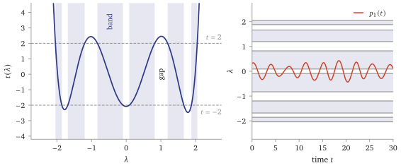
scripts/figures/toda_bands.py asserts the edges constant to and equal to the roots of ).At the equilibrium, all equal and all , every and one finds , with the Chebyshev polynomial: it touches at every turning point, all gaps are closed, and the spectrum is the single band of the free tight-binding model. Outside the loci where a gap collapses, which have codimension two (Henrici and Kappeler, §2 cited), all gaps are open; a special excitation can leave some closed (a state repeating with a shorter period does).
Example 9.28 (All gaps closed: the equilibrium). At and every , and is the free tight-binding model. Its Bloch waves are plane waves , with and energy . Putting , with the Chebyshev polynomial, . It touches at every turning point, so all gaps are closed and the spectrum is one band . This state is the ring at rest in its centre-of-mass frame, drifting with speed . Outside codimension-two loci every gap is open (Henrici–Kappeler, cited), but a special excitation need not open them all (for , a state repeating with period has , the two-site trace, and two of its three gaps stay closed). A gap is the spectral trace of motion relative to the drift, as the actions below make quantitative. At this state the are dependent. By the cyclic symmetry every moves all particles alike, and it changes no momentum, since (the see only differences of positions) and the terms are equal. So every flow is the drift, the span one direction, and for the cannot be independent.
The curve as a two-sheeted cover.
Above each lie two points of , and , which coincide exactly at the band edges. So is two copies of the -plane (the sheets) glued along cuts joining the band edges in pairs; crossing a cut exchanges and (Figure 9.7). With all gaps open, branch points and cuts give a closed surface with handles: genus (Babelon–Bernard–Talon, §6.2 cited), the dimension of the tori of Theorem 9.11. The actions below say why.
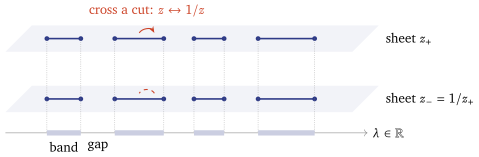
A warning on names. Babelon–Bernard–Talon exchange the letters: their is our , their our , their our , and their particles our (so their genus is our ).
Spectral duality: one curve, read two ways
Proposition 9.26 matched the two eigenvalue problems as sets. The polynomial identity is sharper.
Theorem 9.29 (Spectral duality). For and all , , (9.27) The left side is the characteristic polynomial of the Lax matrix, whose spectral parameter is ; the right side is the characteristic equation of the monodromy matrix, whose spectral parameter is . They define the same curve .
Proof. Expand the determinant over permutations . The matrix is tridiagonal apart from its corners, at and at . A term using the corner and not the one must map and, to stay within the band, for every : the -cycle, of sign , whose term is by (8.11). Likewise the other corner alone gives , and every other term uses both corners or neither and does not involve . So with independent of . Fix and choose with . Then , so is an eigenvalue of , so by Proposition 9.26 . Hence .
The merged matrix satisfies (9.27) too (scripts/check-l10-algebra.py, , symbolic).
Two spectral parameters, one curve.
, the Bloch–Floquet multiplier, lives in the corners of the matrix . Fix : points of , the eigenvalues of . is an -sheeted cover of the -plane.
, the energy of the Bloch wave, is the spectral parameter of the site matrices. Fix : points of , the eigenvalues of . is a two-sheeted cover of the -plane.
The eigenvalue of one Lax matrix is the spectral parameter of the other. The Flaschka normalisation was chosen so that this holds with no factor.
Figure 9.8 draws the -sheeted reading over the unit circle : the familiar band diagram of a crystal. A vertical line meets it in points, a horizontal line inside a band in .
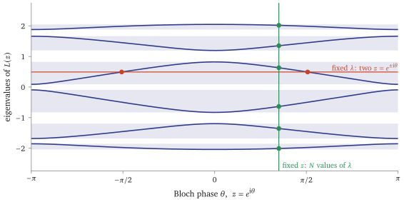
toda_bands.py asserts both, and (9.27) at sampled points).Duality pays off at once.
Corollary 9.30 (Bands and gaps). (i) , so the coefficients and the integrals of §8.6 determine each other, and the are in involution. (ii) wherever . Hence the real line consists of exactly bands, on each of which runs monotonically from to , separated by gaps, some of which may be closed.
Proof. (i) is (9.27) at , and Newton’s identities express the power sums of the eigenvalues through the coefficients of the characteristic polynomial, and back. (ii) At a point of a band interior, with , so the eigenvalue of the Hermitian is simple by Proposition 9.26, and it is a simple root of by (9.27). The count of bands follows, as below.
Proof of (ii) in full. Let with , and . Since , the eigenspace of for is one-dimensional, so by Proposition 9.26 so is that of for . is Hermitian, so is a simple root of , and . So on each maximal open interval where the polynomial is strictly monotone; the interval is bounded, since , and at one end and at the other. Each such interval therefore contains exactly one solution of for each . There are exactly solutions, the eigenvalues of , all simple, so there are exactly such intervals: the bands. Between consecutive bands lie the gaps, closed where two bands touch.
What does and does not buy
An honest remark: gives no new integrals. Expanding (9.27) with Newton’s identities, The -dependence is carried by , a constant by (8.11): holds exactly the integrals had. Contrast Manakov’s parameter in §8.11, which recovered a missed integral.
Where the spectral parameter is indispensable. In the formulation: all integrals are the coefficients of one trace, and without the site matrices carry nothing. In the bracket: (9.9) compares with , and without it there is no composition along the ring; Lecture 14 quantises exactly this, with operator-valued, in place of (9.9), and generating a spin-chain Hamiltonian. And in the geometry: the actions of the tori of Theorem 9.11 are periods of the curve.
Action variables from the curve.
When all gaps are open, the curve has closed loops that stay over the real axis (a closed gap collapses its loop to a point): above the -th gap, both roots are real, and the loop runs along the gap on one sheet and back on the other, crossing between them at the two band edges (Figure 9.9). Call it .
Proposition 9.31 (Actions from the gaps cited). On a regular torus of Theorem 9.11 with all gaps open, the loops correspond to a basis of cycles of the torus in the sense of Lecture 5, and the action variables (6.1) of the relative motion are (9.28) (Flaschka and McLaughlin 1976; in this normalisation, Henrici and Kappeler 2008, Definition 3.1 and Appendix A. The separated variables behind it are Babelon–Bernard–Talon, §§6.5–6.6.)
The second form follows by integrating by parts, with over a gap and oriented so that . A closed gap has zero action; a wide gap means a large amplitude. The proof needs separated variables and the Riemann surface of , which this course does not build. scripts/check-l10-algebra.py checks (9.28) for near equilibrium, where to leading order, (relative error below ), and the example below does by hand.
Example 9.32 (The two-particle ring). Take , with and , a canonical pair, and the mean momentum (not , the permutation operator). Then with relative energy : a particle in a well. From (9.4), with , There is one finite gap, , where , and there is the with . So the right side of (9.28) is : the area of the region in the -plane, divided by . Rename as : it is the area enclosed by the orbit in the -plane over , which is . On the slice we have , so this is the action of Definition 6.1. The same region, sliced two ways.
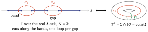
This is the sense in which the genus of equals the dimension of the tori: each open gap is a handle of the curve and a circle of the torus, and its width measures how hard that circle is excited. Theta functions on then give the motion itself in closed form (Babelon–Bernard–Talon, §6.4 cited), which we do not pursue.
Summary
- All integrals at once. The monodromy and the transfer matrix (Definition 9.1); its coefficients include (9.5), and they are Lecture 8’s integrals reorganised, (9.6).
- Tensor legs. has entry ; different legs commute as matrices (Remark 9.3).
- One identity for one site. The quadratic Sklyanin bracket (9.9) composes along an ultralocal chain (Theorem 9.7), and its trace gives (Corollary 9.8).
- Toda. The site matrix satisfies it with (Proposition 9.9); with the Vandermonde argument, the ring is Liouville integrable (Theorem 9.10), and its regular level sets are (Theorem 9.11). Goal G1 is reached.
- Next. Part II begins: Lecture 10 constructs the Heisenberg chain’s eigenstates by Bethe’s guess, Lecture 14 quantises this lecture’s three moves into commuting transfer matrices, and Lecture 15 diagonalises them and recovers the Bethe equations.
References
Babelon, Bernard and Talon, Introduction to Classical Integrable Systems, ch. 2–3 (the Sklyanin bracket) and ch. 6 (the periodic chain, its monodromy matrix and its spectral curve); Faddeev and Takhtajan, Hamiltonian Methods in the Theory of Solitons, Part I ch. 1 (the classical -matrix and the transition to the quantum case); H. Flaschka and D. W. McLaughlin, Prog. Theor. Phys. 55 (1976) 438 (the actions from the gaps). Conventions. Babelon–Bernard–Talon exchange the letters and , and conventions for the sign of differ between all three; see the third caveat.
End of Lecture 9
Why the integrals commute: the Toda ring is integrable
Lecture 9 · Contents
Keyboard
- → Space PgDn
- next screen, stopping before an equation, figure or statement it would cut
- ← PgUp
- previous screen
- ↓ ↑ wheel
- scroll freely
- Home End
- the start or the end
- S
- Full ↔ Spine, keeping your place
- T
- Think first on or off
- R
- reveal the next hidden proof
- C
- Core only on or off
- G
- contents: jump to a section or a statement
- + −
- text size
- D
- light or dark
- F
- full screen
- P
- pen on or off: draw on the text
- E
- erase the ink on the screen
- Z double-click
- enlarge an equation, figure or table; Z again for the next
- L
- laser pointer on or off
- B .
- blank the screen
- M
- move the toolbar: right, bottom, left, top
- ?
- this help
- Esc
- close a panel