Lecture 11
The Lieb–Liniger gas
Course map: G3, step 1 (the model). The method of Lecture 10 works for particles on a line. Bosons with a contact interaction collide pairwise, each collision multiplies the wave by a phase, and the Bethe equations follow as before — this time with a complete proof that the wavefunction is an eigenfunction. For repulsive contact every root is real, and every set of quantum numbers gives exactly one state. This is the gas of the quantum Newton’s cradle, and the model whose thermodynamics Lecture 16 and Lecture 17 compute.
11.1 The question
Lecture 10 solved a lattice model. Lecture 0 asked why a one-dimensional gas might not thermalise, and pointed at the gas of the cradle. So the question is
does the Bethe ansatz solve an interacting gas — and why only in one dimension?
Yes, for bosons with a repulsive contact interaction (Theorem 11.3), with real roots (Proposition 11.4) and one state per set of quantum numbers (Proposition 11.5); and only in one dimension, because only there do two-body collisions keep the set of momenta (§11.5).
11.2 The gas
identical bosons move on a ring of length and interact only when they touch: (11.1) This is the Lieb–Liniger model (1963), repulsive for , in units : a free particle of momentum has energy and velocity .
It is the gas §0.2 promised. In the thin tubes of the quantum Newton’s cradle (Figure 2) the transverse motion is frozen, and the atoms’ short-range interaction becomes, along the tube, a delta of a strength fixed by the scattering length and the tube width (Olshanii 1998) cited. Between collisions the particles are free; the delta imposes a condition wherever two of them meet.
11.3 Two bosons
The contact condition
For two particles use the centre of mass and the separation . Then (11.2) Integrate over and let : . ( itself must be continuous: a jump would put a into that nothing cancels.) So the -derivative jumps by . For bosons is even in , its derivative odd, and the jump is twice the one-sided value. With this is the contact condition (11.3) A symmetric is fixed by its values on , so the problem is: solve the free equation on , subject to (11.3) on its edge (Figure 11.1).
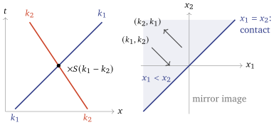
The two-body S-matrix
On try, as in Lecture 10, (11.4) Both waves solve the free equation with the same energy; only the contact condition is left.
Proof. At both waves are , and brings down from the first and from the second. With the condition is , so .
is Proposition 10.1’s formula at . No rapidity is needed: by Galilean invariance, which the lattice lacks, the phase depends on the momenta only through their difference. Its properties:
for real , and . Write (11.6) (Figure 11.2, left).
: with equal momenta and the wave vanishes — a Pauli principle for bosons, which nobody put in.
As at fixed , : the wavefunction vanishes where two particles meet, and these hard-core bosons have the energies of free fermions (Girardeau 1960), the Tonks–Girardeau gas. On the ring the fermions obey , periodic for odd and antiperiodic for even , and this is what “free fermions” means below. As at fixed , : free bosons. (At , for every , so this limit is not uniform in .)
Reflection and transmission. Were the two particles distinguishable, with the same interaction, the relative wave coming in from would be partly transmitted to and partly reflected, with amplitudes (the same integration) For identical bosons a transmitted pair and a reflected pair are the same state, both amplitudes feed the one outgoing wave, and .
What the phase does: a displacement
A plane wave has no position, so superpose: a narrow spread of around and of around , the faster particle on the left. A packet sits where its phase is stationary in the momentum. In the incoming term the phase is , stationary at . In the outgoing term it is , and , so after the collision sketched (11.7) Each momentum comes out on a line parallel to its incoming one: the line carrying the larger momentum is shifted by , the other by — in the centre-of-mass frame, both particles are delayed (Figure 11.2, right, checks this against numerically superposed exact solutions).
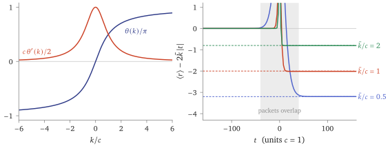
scripts/figures/lieb_liniger.py asserts both.)11.4 bosons
The fundamental domain
Cut the ring at an origin, so that . The planes cut this cube into sectors, one for each order of the particles; periodicity glues cyclically related sectors, which is where the Bethe equations will come from. A symmetric is fixed by its values on the fundamental domain , whose images under permutations are the other sectors (Figure 11.3); it has walls, .
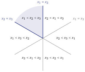
Definition 11.2 (Eigenfunctions of the delta gas). A symmetric, continuous function , periodic with period in every coordinate and smooth up to the walls within each sector, is an eigenfunction of (11.1) with eigenvalue if inside every sector, and on every wall , approached from the side , .
The wall condition is §11.3’s, wall by wall. Rigorously is defined as a self-adjoint operator through its quadratic form, in which the places where three particles meet have measure zero and impose nothing (the KLMN theorem; Reed and Simon, vol. II, §X.2) cited.
The Bethe wavefunction
On the fundamental domain Bethe’s ansatz is Equation (10.14) with momenta for rapidities: (11.8) one factor for each pair of momenta that has exchanged.
Theorem 11.3 (Lieb and Liniger 1963). Let be pairwise distinct, with no two differing by , and let them satisfy the Bethe equations (11.9) Then the symmetric extension of (11.8), if it is not zero, is an eigenfunction of the delta gas on the ring in the sense of Definition 11.2, with (11.10)
Proof. Inside the sectors every term is a plane wave of energy . On the wall pair each with , which exchanges , , and , . On the wall the two terms share an exponential, which no other term has, and together they are a two-body wave in times a factor free of . By Proposition 11.1 the contact condition holds if and only if for every ; the product in (11.8) gains or loses exactly the factor of the pair , which is either way since . The other walls are images of these, and the condition of Definition 11.2 is symmetric, so it goes with them. Periodicity, , is the periodicity step of Theorem 10.2 verbatim: moving from last place to first passes it once past every other momentum, giving , which is (11.9).
All roots are real, and each set of quantum numbers gives one state
The Heisenberg chain has complex roots, strings that make bound states (a reading of Lecture 10). Repulsion forbids them.
Proposition 11.4 (Real roots). For , every solution of (11.9) is real.
Proof. Let have the largest imaginary part, , and suppose . The left side of (11.9) has modulus . On the right, for every , and for real because ; so every factor has modulus at least , a contradiction. Hence . The same argument at the smallest imaginary part, with every inequality reversed, gives the smallest imaginary part . So all are (Korepin, Bogoliubov and Izergin, §I.2).
With real roots take logarithms, using : (11.11) the signs going into (, so the term is harmless). Summing over , the ’s cancel in pairs and .
Proposition 11.5 (Yang and Yang 1969). For and any real , (11.11) has exactly one solution. If then ; in particular distinct quantum numbers give distinct roots, and equal quantum numbers give equal roots.
Proof (★). Let , an even function growing at most linearly. Then (11.11) says for whose Hessian is : times the identity plus a sum of positive semidefinite matrices, since . So is strictly convex and grows like ; it has exactly one critical point, its minimum. For the order, subtract the equations for and : . Since increases, the left side has the sign of .
The reason: (11.11) is the gradient of a strictly convex function of , which has exactly one minimum.
So for the Bethe states are labelled exactly by sets of distinct , one real solution each; coincident roots come only from coincident ’s, and then kills the vector. These are the quantum numbers of free fermions, the limit . That the Bethe states are all the eigenstates is here a theorem (Dorlas 1993, who also proves them orthogonal) cited, unlike for the Heisenberg chain (a reading of Lecture 10). The ground state is the most compact set, , at every (Yang and Yang 1969) cited; Figure 11.4 follows its roots.
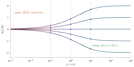
scripts/figures/lieb_liniger.py asserts the equations and both limits; random starts agree at the three marked couplings.)Rapidities. On a ring the particles never become free, yet every eigenstate carries a set , the rapidities, which enter and as if they were. The Bethe states form an orthogonal basis (Dorlas 1993) cited, so a state’s weight on each set is constant in time. That alone decides nothing about relaxation: the weights on the eigenstates of any Hamiltonian are constant. The distribution of §0.2 is a coarser object. Lecture 16 turns a large set into a density of rapidities. Lecture 19 shows, for the Ising chain, how conserved mode occupations fix a non-thermal steady value of a local observable, and Lecture 20 how a complete family of conserved charges fixes the rapidity density of a uniform gas. In the trap of the cradle that density is not conserved: Lecture 20 follows its approximate motion, a shape that keeps returning.
11.5 Why one dimension
§0.2 counted. For two equal masses, momentum and energy are two equations for two outgoing momenta, solved only by the incoming pair or its exchange (Proposition 0.1). Quantum mechanically the same holds for any short-range pair interaction, once the particles are free again: the outgoing wave of two particles contains only the momenta , and scattering fixes nothing but amplitudes.
For three particles the count fails: two equations for three unknowns leave a circle of outgoing momenta, the six rearrangements being six points on it. A generic three-body collision sends waves out over the whole circle — diffraction — which is how a one-dimensional gas can thermalise (Sutherland, §2.2). Non-diffraction is not free. It is what the Bethe wavefunction asserts — in (11.8) only rearrangements of the incoming momenta ever appear — and Theorem 11.3 proves that the delta gas has it. One caution: the two-body count uses ; on a lattice even two magnons are not forced by kinematics (§10.4, at ).
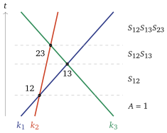
In Figure 11.5 each crossing multiplies the amplitude by one . Had the lines crossed in the other order, the same factors would come in another order, and nothing would change: for bosons without labels three-body consistency is automatic. It stops being automatic when a collision can do more than multiply by a number, which is Lecture 13’s subject.
11.6 What it buys
An interacting gas solved exactly, with a complete proof, and every state labelled by distinct quantum numbers, as for free fermions.
A clean thermodynamic limit. Real roots and one state per set of quantum numbers are what Lecture 16 and Lecture 17 need: the roots become a density, with no strings to track.
Rapidities that label every state, which Lecture 16 turns into a density: conserved in a uniform gas, where Lecture 20 shows what it fixes (Lecture 19 does the same for the Ising chain’s occupations), and moving in the cradle’s trap, where Lecture 20 follows it.
11.7 Caveats, in one place
Status. Theorem 11.3 is proved, wall by wall: unlike on the lattice, where three adjacent spins are a real configuration, the walls of Definition 11.2 never meet in the conditions. Proposition 11.4 and Proposition 11.5 are proved. Completeness and orthogonality of the Bethe states (Dorlas 1993), the ground state’s quantum numbers (Yang and Yang 1969) and the delta as a model of the tubes (Olshanii 1998) are cited.
Repulsion is needed. For attractive the argument of Proposition 11.4 fails: complex roots appear, in strings, as bound states of bosons (McGuire 1964). That gas is not treated.
11.8 Solving the equations
Two particles by hand. Put with . Then , and the first equation of (11.9) becomes , one equation for ( gives the zero vector). Its left side increases from , so each allowed right side gives one root, and . For the ground state has : as (free fermions, ) and as . The check script diagonalises two bosons on a ring of sites, , with , at , extrapolates in , and finds the twelve lowest levels to within of these.
Numerically, use damped Newton on (11.11): its Jacobian is the Hessian of the convex function of Proposition 11.5, positive definite, so every step is well defined; halve the step until the residual decreases. Start from the free-fermion values .
Strong coupling. For , , and with for the symmetric ground state (11.11) becomes , with error : the gas behaves as free fermions on a ring lengthened by .
Weak coupling. For the roots of the ground state crowd together, but their differences, of order , stay large compared with ; then . The terms add up to exactly for the symmetric ’s and cancel, leaving . With this is , Stieltjes’ characterisation of the zeros of the Hermite polynomial (Gaudin §4.3). Figure 11.4 shows both limits.
Summary
- The gas: bosons on a ring with a contact interaction (11.1), the gas of the quantum Newton’s cradle.
- Two bosons: the contact condition gives the phase , (Proposition 11.1).
- bosons: the Bethe equations (11.9), with a complete proof (Theorem 11.3); for every root is real (Proposition 11.4), and each set of quantum numbers has exactly one solution (Proposition 11.5).
- Why one dimension: two-body collisions keep the set of momenta, and the Bethe wavefunction shows that three-body collisions do not diffract.
- Next: Lecture 12 watches the same non-diffraction in classical scattering, on the open Toda chain.
References
E. H. Lieb and W. Liniger, Phys. Rev. 130 (1963) 1605; C. N. Yang and C. P. Yang, J. Math. Phys. 10 (1969) 1115; M. Olshanii, Phys. Rev. Lett. 81 (1998) 938; T. C. Dorlas, Commun. Math. Phys. 154 (1993) 347; Korepin, Bogoliubov and Izergin, Quantum Inverse Scattering Method and Correlation Functions, §I.2; Sutherland, Beautiful Models, §§2.2, 4.2; Gaudin, The Bethe Wavefunction, §4.3.
Lecture 11 · Contents
Keyboard
- → Space PgDn
- next screen, stopping before an equation, figure or statement it would cut
- ← PgUp
- previous screen
- ↓ ↑ wheel
- scroll freely
- Home End
- the start or the end
- S
- Full ↔ Spine, keeping your place
- T
- Think first on or off
- R
- reveal the next hidden proof
- C
- Core only on or off
- G
- contents: jump to a section or a statement
- + −
- text size
- D
- light or dark
- F
- full screen
- P
- pen on or off: draw on the text
- E
- erase the ink on the screen
- Z double-click
- enlarge an equation, figure or table; Z again for the next
- L
- laser pointer on or off
- B .
- blank the screen
- M
- move the toolbar: right, bottom, left, top
- ?
- this help
- Esc
- close a panel