Lecture 17
Dressing, excitations and the thermodynamic Bethe ansatz
Course map: P4, and G3 completed. Lecture 16 put the ground state into the thermodynamic limit. This lecture dresses it and heats it. One linear operator, dressing, turns the bare energy of an added particle into its cost and the derivative of its bare momentum into the derivative of its momentum, and gives the gas its two branches of excitations and its speed of sound. Above zero temperature, counting the ways to fill the vacancies gives an entropy, and minimising the free energy against it gives one nonlinear integral equation, the Yang–Yang equation, whose solution is the gas’s exact equation of state.
17.1 The question
Lecture 16 found the ground states. Physics happens above them. So the question is
what are the excitations, and what is the equation of state at any temperature?
The answer: dressing (Definition 17.1) gives an excitation’s energy and the derivative of its momentum (Proposition 17.2), which gives Lieb’s two branches; at the Yang–Yang equation (Theorem 17.7) gives the pressure. The worked example is the gas at .
17.2 Dressing
Every question asked of a Bethe state in the thermodynamic limit has the same shape. Adding one particle to the sea moves every other root a little, so the change in any extensive quantity is the particle’s own contribution plus the backflow. One linear operator does the bookkeeping for all of them.
Definition 17.1 (Dressing). Let be the filling fraction, (at , the indicator of the sea). The dressed is the solution of (17.1) with the model’s kernel (16.6).
The definition is worth its own name because (16.5) is already an instance of it. It is a response, not a total: the dressed bare momentum is not the excitation’s momentum; the momentum comes from integrating .
Proposition 17.2. for any . Now take , so that is the indicator of the sea, and let an excitation have bare energy and bare momentum ; write . If vanishes at the edges of the sea, then , and the excitation’s dressed velocity is (17.2)
Proof (★). Multiply (16.5) by and use : , which is (17.1) for , for any . For the second statement, differentiate (17.1) in and integrate by parts in , using : being an indicator, is plus delta functions at the edges weighted by there. Those vanish exactly when does, and what is left is (17.1) for . The velocity is then the chain rule. Without the edge condition the boundary terms survive, and : for the gas at , dressing and differentiating gives at against . The step also needs : for a smooth the extra term is , a bulk integral that no edge condition kills.
Remark 17.3 (Which momentum, and which way it runs). is the excitation’s own bare momentum, not automatically (16.5)’s counting momentum . For a particle added to the gas the two agree; for the chain they do not, since runs backwards against (Lecture 16) — and the chain’s excitation is not a magnon but a hole, of bare energy , whose momentum runs with . The spinon reading at the end computes it and finds ; reading (17.2) with and instead flips that sign.
Two things fix the object in place. Equation (17.1) is linear with the same kernel for every , so dressing is one operator : a single numerical solve answers every question. And carries all the state dependence — sharp at , a smooth Fermi function at finite temperature (below), position- and time-dependent out of equilibrium (Lecture 20) — with (17.2) the dressed velocity throughout. What does not carry over is the route to it: at the identity comes from differentiating Yang–Yang’s nonlinear equation for the pseudo-energy (Corollary 17.8).
17.3 Lieb’s two branches
The gas has a Fermi sea with edges, so it has two ways to be excited; Lieb found both in 1963, and both come off one pair of functions. The dressed energy and momentum are (17.3) the first being (17.1) for the bare energy and the second Proposition 17.2; the constant — the chemical potential, and in this lecture there is no spectral parameter to confuse it with — is fixed by . That condition does two things at once: it puts both branches at zero energy where they begin, and it is exactly the hypothesis of Proposition 17.2, so the velocity formula applies. Now add a particle just above the right edge, : energy and momentum trace the Type I branch, the Bogoliubov mode (a particle below gives the mirror branch, referred to ). Move a particle from inside the sea to its edge, leaving a hole at : energy and momentum trace Type II, which rises, turns over and returns to zero at momentum sketched: the branches are computed here from (17.3); that they exhaust the elementary excitations is cited (Lieb 1963).
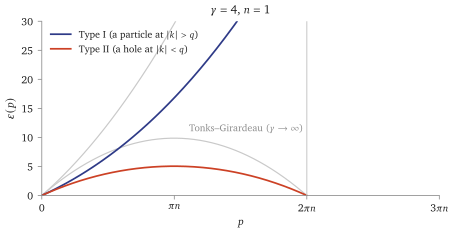
Type II has no counterpart in Bogoliubov theory — it is the exact version of a dark soliton cited: Kulish–Manakov–Faddeev (1976) — and both branches are linear at small momentum with the same slope, the sound velocity that makes the gas a Luttinger liquid.
17.4 Counting
Everything in this lecture rests on one sentence of Lecture 16: a Bethe state is not a list of rapidities but a choice of quantum numbers from the list of vacancies. Choose a subset, solve (16.1), and the roots come out. So counting states is counting subsets — and that is a problem with an answer. For the chain the list is finite, of length , and on the branch where increases the roots occupy distinct members of it (Proposition 16.1, whose second sentence Remark 16.2 showed to be a hypothesis); for the gas the list is all of and is not finite at all. What the count below uses is neither, but the local density of vacancies , which both models have.
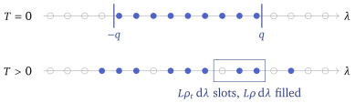
Fix a coarse-graining: cut the rapidity line into cells of width , small on the scale over which varies but wide enough to hold many vacancies. In the cell at there are slots and of them carry roots, where is the number of sites or the length of the box, as in (16.5). The cells are independent, so
Proposition 17.4 (The Yang–Yang entropy). The number of Bethe states compatible with the densities is , and its logarithm is with (17.4) the entropy per site (or per unit length), with the filling fraction of Definition 17.1.
proved as a count, from the hypotheses named below
Proof (★). Stirling gives , so three limits are needed and their order is not free. Cut the rapidity line at and take finitely many cells there. Let : the leading terms are times the bracket in (17.4) and the errors are in each of finitely many cells, hence . Then refine the cells, which turns the sum into the integral. Then let , which converges because the entropy density is integrable. Taking the first two in the other order would not do — with one cell per vacancy the errors are — and without the cutoff the first step never starts, since the gas’s outermost cell holds infinitely many slots. The second form is the first with , .
Remark 17.5 (What the count assumes). For the gas it assumes, first, that every way of filling the slots is admissible, with no further extensive restriction within a cell or between cells; second, that distinct choices give distinct states and exhaust the spectrum — that quantum numbers and solutions are in bijection is Proposition 11.5, and that the states so built are all of them is cited; third, that all choices with the same coarse-grained densities are equally numerous. None of this is proved here. The variational identities below are proved given this count; the saddle-point identification is sketched, and uniqueness is cited. The chain needs a string hypothesis as well (the reading at the end).
17.5 Minimising the free energy
At temperature and chemical potential the equilibrium state minimises the grand free energy per unit length, (17.5) where is the bare energy of one root — for the gas of Lecture 11, for the chain (the reading at the end). Here is the chemical potential, as in Lieb’s branches.
Remark 17.6 ( is not yours to vary). Equation (17.5) is a functional of alone. The hole density is fixed by (16.5), (17.6) The kernel term is the whole of the interaction. Drop it and the variation returns free fermions with the bare dispersion; treat as an independent function and the answer is a Boltzmann factor with no exclusion at all. Both are checked in the script, and the second is the error the section is named after.
proved from Proposition 17.4; that the minimiser gives the true free energy is Yang and Yang’s saddle-point argument, sketched after the proof
Proof. From (17.4), , and turns the two logarithms into and . Substituting from (17.6) and using that is even, The bracket is identically, so the vanishing of the derivative is (17.7). The first equation of (17.8) is the definition of rearranged. For the second, write , use (17.7) to replace in (17.5), and use (17.6) to replace : the two double integrals are equal by the symmetry of and cancel, leaving . The weight is not decoration — it is what the chain’s strings need (the reading at the end), and dropping it would make the chain’s free energy diverge. Finally the stationary point is a minimum: writing , the integrand of (17.4) is , the perspective of the concave and therefore jointly concave in ; and is affine by (17.6). So is concave in , is convex, and the admissible set is convex. That (17.7) has exactly one solution at every , is Yang and Yang’s, and is cited.
Why the minimum is the free energy. The argument is a saddle point. Write the partition function as a sum over sets of quantum numbers, group the sets by their coarse-grained densities, and the sum becomes over the coarse-grained configurations, with of (17.5): the number of terms in each group is by Proposition 17.4 and each contributes . As the sum is dominated by its largest term and , provided the number of groups grows sub-exponentially — which is the usual requirement, and the usual thing that is waved through.
Equation (17.7) is nonlinear — the unknown sits inside a logarithm inside the integral — and that is the price of the temperature. Everything else about it is a gift: one scalar equation, one scalar unknown, and no reference to or to any particular state. And what the second half of (17.8) says is that the minimisation is a Legendre transform. The minimum value of is the grand potential density, ; so is the Legendre transform of the energy density in both and , its partners come back by differentiating, (17.9) and one scalar function of two variables carries the whole thermodynamics. Students lose the last of these by trying to compute from , which is not it: is not an energy.
Corollary 17.8 (Dressing at finite temperature). at every temperature, with of (17.8) in (17.1), and . The effective velocity at temperature is defined, for the gas, by the same ratio as at , (17.10) which reduces to (17.2) when is an indicator. For the chain the denominator must be the excitation’s own bare momentum dressed, not the counting momentum’s (Remark 17.3).
Proof. Differentiate (17.7) in , move the derivative onto by and integrate by parts; the boundary terms vanish because . What is left involves , and the cancels: which is (17.1) for . The second statement is Proposition 17.2, whose first half holds for any ; the third is a definition.
17.6 Two checks
A new equation earns trust by reproducing the two answers already known.
Proposition 17.9 (Impenetrable, and cold). For the gas of Lecture 11, with and :
Proof (★). Both parts need one imported fact: on any bounded set of parameters there is a with , uniformly cited: Yang and Yang (1969). It is what makes integrable with bounded zeroth and second moments, and both proofs use exactly that.
(1) for every , and . With the moments bounded uniformly in , for in a compact set the integral in (17.7) is ; expanding itself then leaves . That is a constant shift of . (2) pointwise and to within uniformly — enough on a compact set, and the tails are handled by the same quadratic bound, not by the uniform bound, whose integral over is infinite. The limit is supported where ; since is continuous and strictly increasing in cited: Yang and Yang (1969), that set is an interval, empty at — the vacuum — and otherwise with . On it the limit of (17.7) is , which is (17.3). For , split (17.8) the same way; then follows from and .
Part (1) carries a sentence of physics, and it is the opposite of the one that suggests itself. The shift raises , so the gas has more pressure than the impenetrable one, while hard rods of length give and less: matching, . At large finite the gas is free fermions in a box lengthened by per particle. The Bethe equations say so directly — turns (11.11) into in the rest frame, — and so does Lecture 16’s , which to this order is with . At , the shift accounts for the whole of the by which the interacting pressure exceeds the free-fermion one.
17.7 Solving it
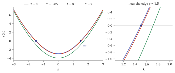
Equation (17.7) has no closed-form solution and does not need one: it is a fixed-point equation, and the obvious iteration works. It also has one fewer parameter than it looks: substituting and makes every cancel between and , so that and depend on alone. One plot is the whole equation of state.
Proposition 17.10 (The iteration contracts). Let be the right side of (17.7). If along the iteration then .
Proof (★). , and in both models — the one place in this lecture where the sign of (Lecture 16) does not matter. So the cancels and the factor is .
The linearisation being differentiated here is nothing other than the dressing operator of (17.1), so the equation that answers every question about the state is also the one that says how fast the solver converges.
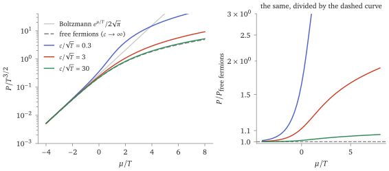
Two features of Figure 17.4 deserve naming. On the dilute side every curve collapses onto : a gas dilute enough is classical, and the coupling cannot be seen. On the degenerate side the curves fan out, and the free-fermion curve is the floor: since , (17.7) gives pointwise and hence at the same and . The impenetrable gas has the least pressure there is, which is the statement of Proposition 17.9(1) seen from the other side.
Equation (17.7) is the equation of state of a real gas: a density profile measured on an atom chip in 2008 is reproduced with no free interaction parameter (the reading at the end).
17.8 What it buys
Dressing, one linear operator for every quantity, and the dressed velocity (Proposition 17.2 and Corollary 17.8): the objects Lecture 20 carries out of equilibrium.
Lieb’s two branches and the speed of sound (Figure 17.1).
The exact equation of state of an interacting quantum gas at every temperature and coupling (Theorem 17.7), checked in both limits (Proposition 17.9) and measured. Goal G3 is reached.
17.9 Caveats, in one place
Status. Proposition 17.2, Theorem 17.7, Corollary 17.8, Proposition 17.9 and Proposition 17.10 are proved, the first, fourth and fifth in readings; Theorem 17.7 rests on the count, whose assumptions (Remark 17.5) are not proved. That the minimum is the free energy is a saddle-point argument, sketched; that the Yang–Yang equation has one solution is cited, as is that Lieb’s two branches are all the elementary excitations.
Two hypotheses in Proposition 17.2. Its second half needs and ; at the identity is derived again, from the Yang–Yang equation (Corollary 17.8).
The effective velocity at is a definition (17.10); that it is a propagation speed is not proved here.
The chain needs strings, and the string hypothesis is false as a statement about individual solutions; its thermodynamics is a reading.
17.10 The chain’s excitations: spinons
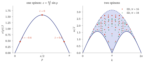
Return to the antiferromagnet and make the cheapest excitation there is: remove one root. The sector is , which by Proposition 16.1 has vacancies for roots — two holes, at — while the magnetisation has gone up by one, . Two objects, one unit of between them: by itself that would also allow a spin and a spin . What settles it is the multiplet structure — at fixed the states form one triplet and one singlet, exactly as two spin- objects do cited: Faddeev–Takhtajan (1981). They are the spinons, and that is the most surprising sentence about the chain: the elementary excitation of a spin chain is not a magnon of spin but half of one, and it cannot be made alone.
Theorem 17.11 (The spinon). Let be even and let a state of the antiferromagnet lie on the branch of Proposition 16.1 — pairwise distinct real roots, increasing — with of them, so that it carries holes, necessarily an even number, and let stay fixed as . In the limit of Theorem 16.3, if the holes sit at then (17.11) with (17.12)
proved from the first-order form of the assumption noted after the proof; the dispersion is that of des Cloizeaux and Pearson (1962)
Proof. With as above, . With holes, (16.4) reads , while for the sea (16.8); subtracting and putting , . Hence, being symmetric, which is (16.7) up to : so . For the momentum, (10.19) gives exactly, and deleting roots from a symmetric filled set leaves , so , and , since at fixed . Summing gives , and is even. Finally integrates to (17.12), and .
The proof is a backflow computation. With the bare magnon energy , putting delta-function holes into (16.4) and inverting dresses the energy of the removed magnon, — and that equation is (16.7) again, so . It runs on one order finer information than Theorem 16.3’s assumption supplies: at fixed the hole density tends to zero, and (17.11) needs . The careful route subtracts the two finite systems and linearises before letting cited: Takahashi §3.4; it gives the same , and finite chains agree (the check script, to ).
The continuum, and what a neutron sees.
A two-spinon state has , , with distinct (the holes sit at distinct vacancies). At fixed , grows as shrinks and falls as one spinon reaches an end of its band.
Corollary 17.12 (The two-spinon continuum). The two-spinon states are dense in (17.13) and fill its interior. Neither boundary is attained: the upper one is the limit , the lower one the limit in which one spinon runs to the end of its band, .
The lower boundary is the des Cloizeaux–Pearson dispersion of 1962, read for thirty years as the spin-wave branch; the upper one shows it is only the edge of a continuum. That is the measurable difference between a spin chain and a magnet: a three-dimensional antiferromagnet scatters neutrons into a sharp magnon line, the spin- chain into a broad continuum, because a neutron flips one spin and therefore makes spinons in pairs — two at least, any even number in principle — which share the energy as they like. Inelastic scattering on KCuF sees such a continuum, and the 1995 measurement was fitted with an approximate two-spinon cross-section, the Müller ansatz. The exact two-spinon contribution, computed later, exhausts about of the integrated intensity; four spinons and more carry the rest cited: Tennant, Cowley, Nagler and Tsvelik, Phys. Rev. B 52 (1995) 13368; Müller, Thomas, Beck and Bonner, ibid. 24 (1981) 1429; Lake et al., Phys. Rev. Lett. 111 (2013) 137205.
Which way does run? Theorem 17.11 could as well have printed : it satisfies just as well, and for a pair of holes at gives the same total, . A symmetric test cannot tell the two apart — which is exactly why one must test an asymmetric pair. Against finite chains with the holes placed asymmetrically the printed orientation is right to at and the other is wrong by . The counterexample lives in the check script.
17.11 Two limits of the entropy, the filling fraction, and the experiment
Remark 17.13 (Two familiar limits of one formula). and both give zero: an empty region and a full one each admit one arrangement. The maximum is per slot at . And (17.4) is the entropy of a set of fermionic modes — one slot, one particle — even though the gas of Lecture 11 is made of bosons. The exclusion is not in the statistics of the particles but in the Bethe equations, which forbid two equal quantum numbers.
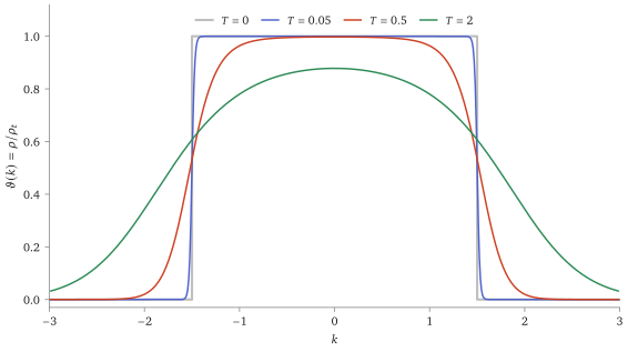
Equation (17.7) is not a model equation of state; it is the equation of state of a real gas. Ultracold Rb on an atom chip, confined so tightly in two directions that only the lowest transverse mode is populated, is the Lieb–Liniger gas of Lecture 11 with set by the transverse confinement. Measuring the in situ density profile of such a cloud, and reading the trap’s slowly varying potential as a local chemical potential , turns one image into a curve of against at fixed . Van Amerongen and co-workers did this in 2008 for a weakly interacting gas on an atom chip, fitting only and : no interaction parameter is free, since follows from the transverse confinement. One complication is instructive — at their temperatures the higher transverse modes are not empty, so what is fitted is : Yang–Yang for the one-dimensional gas, an ideal gas for everything above it. With that, the profiles are reproduced across the crossover from the quasi-condensate to the nearly ideal gas — where mean-field theory has nothing to say cited: van Amerongen et al., Phys. Rev. Lett. 100 (2008) 090402.
17.12 Strings, and the chain’s thermodynamics
Everything so far used only real roots, and for the gas that is a theorem (Proposition 11.4). The chain is different. Lecture 10 already met a solution with and exponentially small in (10.23), and its argument — an imaginary part forces a nearly vanishing denominator — applies to any number of roots.
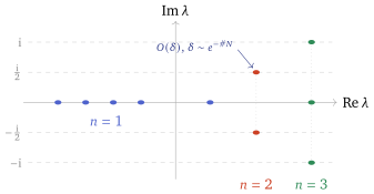
Definition 17.14 (Strings, and the hypothesis). An -string is a set of roots , , with real centre . The string hypothesis is that as the roots of the solutions that matter thermodynamically organise into strings, up to deviations exponentially small in .
cited, and false in detail: Essler, Korepin and Schoutens (1992)
The hypothesis is known to fail. There are “wide pairs” whose imaginary parts are not , and -strings that collapse onto the real axis as grows; Lecture 16 met the tail of the same phenomenon in the pair of real roots sharing a quantum number at (Remark 16.2). What survives — and what the thermodynamics needs — is the counting: the string configurations reproduce the right number of states even where individual solutions are wrong. That is less than it sounds, and this reading returns to it: a partition function weights states by energy, so equal cardinality is not equal free energy. This is an uncomfortable position to be in and it is the honest one.
Bethe–Takahashi.
Put the string of Definition 17.14 into the Bethe equations and multiply the equations of its members together. The exponentially small deviations cancel between a diverging and a vanishing factor, and what is left is one equation per string centre: (17.14) with the scattering phase between an -string and an -string (17.15)
sketched: the cancellation of the deviations is the content, and it is cited (Takahashi 1971)
For this is and (17.14) is Lecture 16’s (16.1). Two consequences follow as they did there, by reading off the values at : since with , the number of vacancies for -strings is (17.16) with the number of -strings and as in Theorem 16.3. The energy follows from the identity for an exact string, together with Lecture 10’s (10.16): an -string of centre carries energy and lowered by . For that is , the bare energy §17.5 asked for.
The chain’s TBA, and the Y-system.
Repeat §17.5 with one density per string length. Put the chain in a field, . An -string lowers by , so the Zeeman energy is : the magnons’ chemical potential is , and it is that takes the place of the gas’s . Nothing else changes except the bookkeeping, and the answer is an infinite coupled system: with , (17.17)
sketched: this is Theorem 17.7’s variation with one density per string length, not redone here
The sign in front of the sum has flipped because (Lecture 16): at , (17.17) is (17.7). Infinitely many equations, each with infinitely many terms, is not progress. It becomes progress because the matrix has an inverse that is almost diagonal: in Fourier variables with , i.e. with the kernel . Applying it collapses (17.17) to
Theorem 17.15 (Takahashi’s TBA for the Heisenberg chain). With and , (17.18) with entering only through .
sketched: the Fourier inversion is checked in the script; the convergence of the truncation is numerical
Three things fall out at once. The driving term now sits at alone, and every other equation couples only to its two neighbours — a chain in the index . The constant in is Lecture 16’s Hulthén ground-state energy (16.9), and it arrives here as , not by assumption. And at the driving vanishes and (17.18) has the constant solution , whence — the free energy of free spins, by a telescoping product.
Remark 17.16 (The Y-system). is the inverse of , and , whose sum vanishes identically. Those two facts use the same symbol for two prescriptions — approached from inside the strip the shifted sum of is a nascent , which is exactly why the operator inverts — so the driving term is not destroyed but re-encoded. For analytic in , applying the operator to (17.18) away from leaves (17.19) The temperature, the coupling and the field have vanished: they survive in the analyticity and the asymptotics alone. The Y-system is universal, and it is where Lecture 15’s reappears: fusing the auxiliary space gives a tower of transfer matrices whose eigenvalues obey the same hierarchy and are generated from a single (15.20). The thermal are not those ratios — the same functional relation has many solutions, and the temperature is in the analyticity — which is the point the reading makes.
In practice one truncates at some and, at zero field, imposes beyond it. At the truncation error falls below by , and the free energy so computed agrees with exact diagonalisation of the finite chain — with a finite chain, where no string ever appears — to five decimals at , and . The check script does exactly that comparison, and it is the strongest evidence this reading offers that the string hypothesis, false in detail, counts correctly — not the strongest there is, since the same equations follow algebraically from the quantum transfer matrix with no string hypothesis at all cited: Essler et al. (2005). Note what it settles. That the string configurations preserve the number of states does not by itself give the free energy, since weights states by energy; it is the agreement of the energies that is the evidence.
17.13 The field’s factor, and where reappears
Two things §17.12 asserted are worth doing properly: the field’s normalisation, which no check of the equations can see, and the promise Lecture 15 made about the T–Q relation, which is worth keeping exactly as far as it is true.
The field. Everything in (17.18) except the boundary condition is blind to : the operator that produced it annihilates the sequence (check script). So the normalisation of survives in exactly one place, and it is the one place no check of the equations can see. Set , where the answer is known. The recurrence has the constant solution , for which , and (17.18) gives . A free spin in has , so and the boundary condition is . Takahashi’s is because his field term is : taking his boundary condition with our Hamiltonian multiplies the zero-field susceptibility by four. As the hyperbolic solution becomes , which is why that is the zero-field truncation.
Where reappears, and where it does not. Fusing the auxiliary space of Lecture 14 to spin gives a tower of transfer matrices , and their eigenvalues obey a T-system: a relation of the shape (17.20) with a known scalar built from the vacuum factors. Put ; then (17.20) at gives , and the satisfy (17.19) provided — a condition on the scalar alone, which the standard satisfies identically (check script). And every fused eigenvalue is generated from a single Baxter together with those vacuum factors: that is the sense in which Lecture 15’s T–Q relation (15.20) generalises cited: Kuniba, Nakanishi and Suzuki (2011) §§6, 8.
Now the warning, which is the reason this is a reading and not a theorem. The so constructed are not the thermal . They cannot be: an ordinary transfer matrix of a finite chain has no temperature in it. At on the reference state the ratio is a non-constant rational function of , negative on an interval, where the thermal solution is the constant . A functional equation does not determine its solution; the temperature enters through analyticity and asymptotics, and the object whose ratios are the thermal is the quantum transfer matrix, a Trotter-limit construction this course does not build cited: Essler et al. (2005), §13.2 and appendix 13.A. What Lecture 15 promised is delivered here at the level of the hierarchy — the Y-system of (17.19) is the T–Q relation’s, seen from the other side — and not at the level of the solutions.
17.14 Why it works, and what it does not prove
Theorem 17.7 minimises a functional. What entitles anyone to believe that the minimum is the free energy?
The saddle-point argument is in §17.5.
Yang and Yang proved what can be proved cleanly: that (17.7) has a unique solution for every , , that is analytic in and and increasing in , and that the resulting is convex — so that the thermodynamics it defines is consistent cited: Yang and Yang (1969). What their argument does not establish is the step before: that the set of Bethe states really is in bijection with the sets of quantum numbers, and that the coarse-graining loses nothing. For the gas, half of the first is a theorem: quantum numbers and solutions are in bijection (Proposition 11.5); that the states so built are all of them is still cited. For the chain even that much rests on the string hypothesis, which is false as a statement about individual solutions. The subject’s position is that the counting is right even so. Part of the evidence is numerical — §17.12’s exact diagonalisation, at the three temperatures it reports, and no further, since a ring of fourteen sites is not the thermodynamic limit at low temperature. The rest is theoretical, and independent: the same equations come out of the quantum transfer matrix without any string hypothesis cited: Essler et al. (2005), §13.2 and appendix 13.A.
There is a second, sharper reason to trust it. The same that minimises is the one that appears in the dressing equation, and Corollary 17.8 makes the dressed velocity a derivative of the free energy’s own ingredients. Thermodynamics and dynamics are answered by one function. Lecture 20 takes that seriously enough to let depend on position and time.
One more caution. is not a bare, state-independent one-particle energy: it depends on and , and only at does it reduce to . What it is is the dressed cost of a particle–hole excitation above the thermal state — moving a root from to costs , backflow included cited: Korepin, Bogoliubov and Izergin §I.8 — which at reduces to the dressed energy (17.3). The trap is the next step: reading as a Boltzmann weight for a particle of energy gets the filling right for the wrong reason, and stops working the moment one asks for a correlation, where the shape of the state and not only its occupations is needed.
17.15 Solving the Yang–Yang equation
The recipe is Lecture 16’s Nyström method (16.15) wrapped in the iteration of Proposition 17.10. Take an -point Gauss–Legendre rule on , start from , and iterate (17.21) then read off , , and — by one linear solve with the same matrix — and every dressed quantity. Three practical points, all of which cost something before they were learnt.
The cutoff and the grid answer to different scales. is set by where dies — by , and read off the interacting , not the bare one. The number of nodes is set by the sharpest feature, and there are two: at low temperature the Fermi edge, of width in rapidity (not , which is its width in dressed momentum), and at small the kernel itself, a peak of width . Large is therefore the easy end — the kernel flattens towards — and small is the hard one, where a rule that does not resolve the peak has a Nyström diagonal that diverges instead of tending to a row integral of one. What is not set by is : taking , as looked natural, put the nodes so far apart that the pressure came out as .
Convergence in is not uniform in . At with the cutoff used throughout (so at and at ), an -point rule is converged to ten digits at , where points give ; at the same points are wrong in the fourth digit, for exactly the reason above. Quote a cutoff with every such number — at the warm -point error is six times larger. As in Lecture 16: run against , and do it at the temperature you mean to use, not at the one where the code was written.
Check the thermodynamics, not the equation. The strongest test costs two extra solves: against and against , with computed from (17.4) and from . These agree to eight digits when everything is right and fail loudly when a factor of is not. They also confirm the equation’s weakest link — comes from a linear solve that never appears in (17.7), so nothing else would catch an error in it.
A worked number. At and the that (17.3) gives for (so , ), the sound velocity is and the low-temperature pressure obeys to four digits at : the Sommerfeld correction with central charge one, which is the Luttinger-liquid statement of Lecture 16’s reading seen from the thermodynamic side.
Finally, the chain. The same iteration solves (17.18), but now is a convolution best done by fast Fourier transform on a uniform grid, the index must be truncated, and the initial guess is the right one because it is the exact solution. Twenty string lengths and a grid of points on give the free energy to five decimals in about six seconds (thirty lengths cost three times that and buy one more decimal), which is enough to put it beside the exact diagonalisation of a -site ring and watch the two agree.
Summary
- Dressing (Definition 17.1): ; , and at with the edge condition (Proposition 17.2).
- Lieb’s branches: a particle above the sea (Type I) and a hole in it (Type II), both linear at small momentum with the speed of sound.
- Counting (Proposition 17.4): a state is a choice of filled vacancies, and its entropy is that of fermionic slots.
- Yang–Yang (Theorem 17.7): minimising gives , a Fermi function of , and the pressure; dressing holds at every (Corollary 17.8).
- Next: Lecture 18 solves the Ising chain by free fermions, the model Lecture 19 needs out of equilibrium.
References
C. N. Yang and C. P. Yang, J. Math. Phys. 10 (1969) 1115; E. H. Lieb, Phys. Rev. 130 (1963) 1616 (Types I and II); M. Takahashi, Thermodynamics of One-Dimensional Solvable Models, Cambridge University Press (1999), chapters 3–5, 7 and 8; V. E. Korepin, N. M. Bogoliubov and A. G. Izergin, Quantum Inverse Scattering Method and Correlation Functions, Cambridge University Press (1993), §§I.4, I.6, I.8; F. Franchini, An Introduction to Integrable Techniques for One-Dimensional Quantum Systems, Springer (2017), §2.9; L. D. Faddeev and L. A. Takhtajan, Phys. Lett. A 85 (1981) 375 (the spinon); F. H. L. Essler, V. E. Korepin and K. Schoutens, J. Phys. A 25 (1992) 4115 (strings); A. H. van Amerongen et al., Phys. Rev. Lett. 100 (2008) 090402 (the experiment).
End of Lecture 17
Dressing, excitations and the thermodynamic Bethe ansatz
Lecture 17 · Contents
Keyboard
- → Space PgDn
- next screen, stopping before an equation, figure or statement it would cut
- ← PgUp
- previous screen
- ↓ ↑ wheel
- scroll freely
- Home End
- the start or the end
- S
- Full ↔ Spine, keeping your place
- T
- Think first on or off
- R
- reveal the next hidden proof
- C
- Core only on or off
- G
- contents: jump to a section or a statement
- + −
- text size
- D
- light or dark
- F
- full screen
- P
- pen on or off: draw on the text
- E
- erase the ink on the screen
- Z double-click
- enlarge an equation, figure or table; Z again for the next
- L
- laser pointer on or off
- B .
- blank the screen
- M
- move the toolbar: right, bottom, left, top
- ?
- this help
- Esc
- close a panel