Lecture 7 diagnosed classical integrability by a picture (Figure 7.5): at the same energy, an orbit of the Toda ring crosses a Poincaré section on a curve, the torus it winds round cut by the section (Figure 7.2), while most orbits of its cubic truncation, Hénon–Heiles, scatter over an area. A quantum system has no orbits to cut. So the question is

The answer: not the number of conserved operators (Proposition A.1) but their locality; and, as a test, the level statistics inside one fully resolved symmetry block — Poisson for XXZ, Wigner–Dyson with a next-nearest-neighbour coupling $J_2=0.5$ at $N=18$ (Figure A.2). The test is one of three working criteria, and no general theorem connects them (§A.5). The worked example is Lecture 19’s chain (19.1).

By Lecture 10’s rule of translation (10.1), $A$ is conserved when $\comm{A}{H}=0$, and two conserved operators are “in involution” when they commute. Every ingredient of Lecture 5’s definition translates except independence.

Every function of the energy is conserved, $\pb{h(H)}{H}=0$, so conserved quantities are never scarce. Liouville’s definition (Definition 5.5) asks for more: $n$ of them whose differentials are linearly independent (Definition 5.1). That is a condition with content. $h(H)$ fails it, since $\dd h(H)=h'(H)\,\dd H$ is parallel to $\dd H$; and independence is what makes a level set $\{F=f\}$ an $n$-dimensional manifold, which, where compact and connected, the theorem proves to be a torus (Theorem 5.7). At most $n$ functions in involution can be independent (Proposition 4.11), so “$n$” is a sharp number.

Take the simplest quantum system that could be a many-body problem: a Hilbert space $\C^{D}$ of finite dimension. A chain of $N$ spins $\tfrac12$ has $D=2^{N}$. Let $H$ be Hermitian with simple spectrum $E_1<E_2<\dots<E_D$ and eigenvectors $\psi_a$, and let $\Pi_a=\psi_a\psi_a^{\dagger}$ be the projector onto the $a$-th eigenline. (The projectors are $\Pi_a$ throughout; $P$ is the permutation operator of Definition 9.4.)

Now try to say what “$D$ independent conserved operators” should mean.

• Linearly independent. By (a), every Hamiltonian with simple spectrum has $D$ of them in involution, $D-1$ after discarding the identity $\sum\Pi_a$ (with degenerate levels, take the projectors of any eigenbasis). A random matrix qualifies as well as the XXX chain of Lecture 10.

• Functionally independent, the classical notion, where $A=f(B)$ counts as dependent, as $h(H)$ did. By (b), if the spectrum is simple then every conserved operator is a function of $H$, and no such Hamiltonian has a single integral beyond $H$ itself, however regular its dynamics. With degenerate levels, as for XXX, the same happens one step up: every commuting family consists of functions of one operator (von Neumann; the reading at the end of this lecture).

• Algebraically independent: no nonzero polynomial relation among them. By (c), not even one operator on $\C^{D}$ is algebraically independent; the projectors satisfy $\Pi_a^{2}=\Pi_a$ and $\Pi_a\Pi_b=0$ besides.

One reading makes every system integrable, the other two make none. The count of commuting operators cannot be the definition, and there is no quantum analogue of functional independence to rescue it: the classical notion was a statement about differentials, and a finite matrix has none. Caux and Mossel (2011) call the counting definition “too naive” for this reason cited.

What survives is not how many conserved operators there are but what they look like in the basis in which the system was written down. The projector onto a typical eigenstate of a chain of twenty spins has nonzero entries all over its symmetry block, a block of dimension up to about $10^{4}$; the Hamiltonian is a sum of twenty terms, each acting on two neighbouring spins. Lecture 19’s local charges (Definition 19.1) make the difference precise: those of range at most $r$ span at most $4^{r}$ dimensions, whatever $N$ (Proposition 19.2), while the commutant has at least $2^{N}$. At any fixed range, then, the local charges fill a fraction at most $4^{r}/2^{N}$ of the conserved operators, which goes to zero as the chain grows. So no family of local charges of one bounded range can be complete; a tower whose ranges grow, like XXX’s (Lecture 15’s reading), needs a separate count, and on a ring of $N$ sites it has only about $N$ members. Locality — not number — is what can tell one Hamiltonian’s conserved quantities from another’s.

Write $P_n:=P_{n,n+1}$ for the permutation of two neighbouring sites, so that Lecture 10’s Heisenberg Hamiltonian is $H=\frac J2\sum_n(P_n-1)$ (10.2), a local charge of range $2$.

$Q_3$ is genuinely new: it is not a polynomial in $H$ (the tutorial shows this by a reflection), and Lecture 15’s reading finds it in the second logarithmic derivative of the transfer matrix, and sketches the tower above it. And the proof is fragile. Add a next-nearest-neighbour coupling $J_2\sum\mathbf S_n\cdot\mathbf S_{n+2}$ — the $J_1$–$J_2$ chain — and both cancellations fail, and a computer search at $N=8,9$ finds no range-$3$ conserved charge beyond $H$ and the total spin (the tutorial). Make the chain anisotropic instead (XXZ) and (A.2) fails too, but a modified range-$3$ charge exists: XXZ is integrable. Grabowski and Mathieu proposed the existence of one range-$3$ charge beyond the Hamiltonian as a test of integrability; it is a conjecture cited.

Let $E_1\le E_2\le\dots$ be the eigenvalues of $H$ in one symmetry sector, a notion made precise below, and $s_n=E_{n+1}-E_n$ the spacings. The density of levels varies across the spectrum, so before spacings from different places can be compared they are unfolded: replace each $E_n$ by the smoothed count of levels below it, so that the mean spacing is $1$ everywhere. The histogram $P(s)$ of unfolded spacings is the object.

Uncorrelated levels. If the levels were independent random points of unit density, the chance that an interval of length $s$ contains none of them would be $e^{-s}$ (the limit of $(1-s/L)^{L}$ for $L$ points in length $L$), and the spacing distribution is $$P_{\mathrm P}(s)=e^{-s}\qquad\text{(Poisson).}$$(A.3) Its maximum is at $s=0$: nearly degenerate pairs are common.

Levels that repel. Now let the Hamiltonian be a generic real symmetric matrix, with no structure. For two levels the whole story is visible.

The factor $s$ is the whole point. A degeneracy needs two conditions, $a=b$ and $c=0$, and two conditions on a random point of the plane are met with probability zero and nearly met only rarely: level repulsion, $P(s)\to0$ as $s\to0$. For large GOE matrices the spacing distribution is not exactly (A.4), but close to it (the first reading at the end of this lecture measures how close). “Wigner–Dyson statistics” means this shape.

Why should an integrable system be Poissonian and a chaotic one look like a random matrix? Two conjectures say so, supported by much evidence and proved in neither generality: Berry and Tabor (1977) for integrable systems and Bohigas, Giannoni and Schmit (1984) for chaotic ones cited; spin chains were tested from Poilblanc et al. (1993) on. The picture to keep: in an integrable system every level carries quantum numbers, one per conserved charge, and levels with different labels do not mix, so their spacings are uncorrelated; in a chaotic system nothing labels the levels, and every pair repels (the reading at the end of this lecture).

Unfolding needs a fit and a choice of what to discard at the edges. A statistic that needs neither is the ratio of consecutive spacings (Oganesyan and Huse 2007), $$r_n=\frac{\min(s_n,s_{n+1})}{\max(s_n,s_{n+1})}\in[0,1],$$(A.5) which does not see the local density because it is a ratio. For Poisson levels its mean is $$\langle r\rangle_{\mathrm P}=2\ln2-1\approx0.386$$(A.6) (the tutorial at the end of this lecture); for the GOE, $\langle r\rangle\approx0.531$ (Atas, Bogomolny, Giraud and Roux 2013, who find $0.5307$ numerically for large matrices and $4-2\sqrt3\approx0.536$ from $3\times3$ ones) cited. One number, between $0.386$ and $0.531$, is the whole diagnosis.

The first experiment everyone does gives the wrong answer. Take a chain that nobody believes to be integrable and histogram its spacings (Figure A.1, left): Poisson.

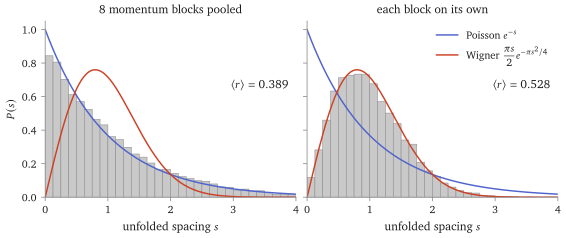
The reason is block structure. If $H$ commutes with a symmetry — here the translation $\tau$ — it is block diagonal in the symmetry’s eigenbasis, one block per eigenvalue (per momentum $k$). Levels in different blocks sit in different blocks of a matrix: they never mix, so they do not repel, and a list that interleaves several blocks’ spectra is a superposition of independent sequences. Superpose enough independent sequences and the result is Poisson whatever each one was — the same reason independent points are Poisson. (Two GOE spectra superposed already give $\langle r\rangle\approx0.43$; eight give $0.39$; check-l13-algebra.py.) So a symmetry left unresolved fakes integrability. The cure is to diagonalise one block at a time and collect statistics inside each.

Which symmetries. Here: translation (momentum $k=2\pi j/N$), the total $S^{z}$, the spin flip $S^{z}\to-S^{z}$, the reflection $k\to-k$, and for isotropic chains $\SU(2)$. A block is resolved when no remaining unitary symmetry acts within it (an antiunitary one may, and fixes the reference ensemble; the first reading); $S^{z}=1$, $0<k<\pi$ and anisotropy achieve it, since the flip and the reflection each move such a block to a different one. That argument is the proof. The generator adds a necessary check, not a sufficient one: no two levels in any block coincide (no spacing below $10^{-8}$ of the mean). A reader repeating the experiment should do both.

The chain is Lecture 19’s (19.1), at $\XXZ=0.55$. At $J_2=0$ it is the XXZ chain, which the algebraic Bethe ansatz solves (Lecture 15’s reading); for $J_2\ne0$ it is not known to be integrable, and Figure A.2 shows why nobody expects it to be.

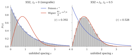
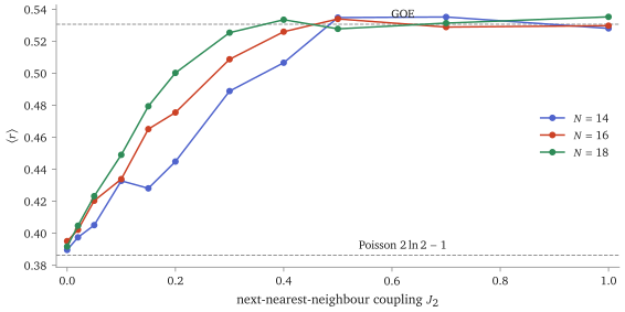
Figure A.3 sweeps $J_2$. The mean ratio leaves the Poisson value as soon as $J_2$ is switched on; at $N=18$ it reaches the GOE value by $J_2\approx0.4$, at $N=14$ only at larger coupling, and the crossover is sharper for the longer chain. Whether an arbitrarily small $J_2$ makes an infinitely long chain chaotic is a real question, and the figure cannot answer it; §A.6 returns to it.

The working criteria of quantum integrability, as used in practice and on the path of this course:

1. (T)

   Transfer-matrix charges. A family of commuting transfer matrices $t(\lambda)$, built from a solution of the Yang–Baxter equation (Lecture 14), whose logarithmic derivatives give a tower of local conserved charges (Lecture 15 and its reading).

2. (S)

   Non-diffractive scattering. When particles are far apart, their momenta are conserved as a set, and many-body scattering factorises into two-body events — the quantum form of Lecture 12’s Theorem 12.2, and Sutherland’s definition (Lecture 10, Lecture 11, Lecture 13).

3. (P)

   Poisson statistics, in fully resolved symmetry blocks.

They are criteria, not a definition, because no general theorem connects them, and there are systems where one holds without another.

• Charges without (P). The Haldane–Shastry chain, whose exchange falls off as the inverse square of the chord distance, has an explicit commuting family of conserved charges (Talstra and Haldane 1995), though not local ones: they are sums over pairs, triples, … of sites. Its level statistics are neither Poisson nor Wigner–Dyson (Finkel and González-López 2005, quoted by Caux and Mossel) cited. The harmonic oscillator is not Poisson either (the reading on Berry and Tabor).

• (P) without (T). A strongly disordered chain in the many-body localised regime shows Poisson statistics and has no transfer matrix; it has quasi-local conserved quantities of its own, but whether that regime survives in infinitely long chains is contested (Abanin, Altman, Bloch and Serbyn 2019; Šuntajs, Bonča, Prosen and Vidmar 2020) cited. And, as Figure A.1 showed, (P) can be produced by carelessness alone.

• (S) needs room. Non-diffraction concerns particles that separate — gases on a line, dilute excitations of a chain — and says nothing directly about a finite spectrum (Caux and Mossel) cited.

Symmetry is not integrability, in either direction. The $J_1$–$J_2$ Heisenberg chain has all of $\SU(2)$ and translation, so its levels come in large degenerate multiplets; yet within blocks of fixed total spin and momentum its statistics are Wigner–Dyson ($\langle r\rangle=0.53$ at $J_2=0.7$, $N=18$, total spin $1$; check-l13-algebra.py), and a search at that coupling ($N=8,9$) finds no range-$3$ charge beyond $H$ and the total spin (the tutorial). Conversely the anisotropic XYZ chain, $\sum(J_xS^{x}S^{x}+J_yS^{y}S^{y}+J_zS^{z}S^{z})$ with three different couplings, has no continuous symmetry at all and is integrable, by a commuting family of transfer matrices (Baxter, Exactly Solved Models, §10.14) cited. Degeneracies count symmetries; integrability is something else.

On the path, Lecture 14 constructs commuting transfer matrices for XXX and for quantum Toda; for XXX, Lecture 15 obtains the Hamiltonian from their logarithmic derivative, and its reading sketches the local tower. The Ising chain’s charges are constructed directly, with no transfer matrix (Lecture 18’s reading, Proposition 19.8). None of the criteria is assumed to imply another.

Lecture 7 diagnosed classical integrability by a picture: curves or scattered dots in a Poincaré section (Figure 7.5). Figure A.4 sets it beside this lecture’s. No theorem relates the two rows — one is a property of orbits, the other of a spectrum — but they play the same role, and the two conjectures above claim that they agree where both make sense.

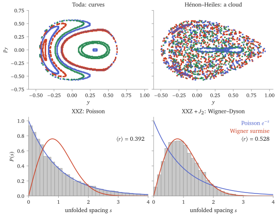
The mirror goes one step further. Classically, a weak perturbation of an integrable system does not destroy it at once: most tori survive (KAM, Theorem 7.8), and chaos grows from the resonances. The quantum question is what Figure A.3 raises and cannot settle: does a weakly broken integrable chain keep a memory of its charges? For a while it often does — the prethermal plateau of Remark 20.2 — and whether it does in a controlled sense is the quantum KAM question, which that remark leaves open.

• A test anyone can run: $\langle r\rangle$ inside fully resolved blocks, $0.386$ against $0.531$ (Figures A.2 and A.3).

• Why it is not a definition: counting decides nothing (Proposition A.1), and no general theorem connects the criteria.

• The quantum mirror of Lecture 7, related by conjecture, not by theorem; and, in a reading, the tori globally, left open by Lecture 5 and Lecture 6.

• Status. Proposition A.1 and Proposition A.3 are proved; Theorem A.2 and $\langle r\rangle_{\mathrm P}=2\ln2-1$ are proved in the tutorial. The two conjectures, the GOE value of $\langle r\rangle$ and the charges of Haldane–Shastry and XYZ are cited. Every statement about one chain at one size — the figures, the charge search — is numerical, at that size only.

• Resolved means proved resolved, by an argument about the symmetries; no coincident levels is a necessary check, not a sufficient one.

• The limit is open: Figure A.3 does not settle whether an arbitrarily small $J_2$ makes an infinitely long chain chaotic.

• Classical and quantum are not one definition. The one bridge the course proves, Lecture 14’s limit $\hbar\to0$, takes quantum Toda’s $RTT$ relation to Lecture 9’s bracket: one structure in one model, not one definition into another. Spin chains have no classical limit at fixed $N$ (the reading on Berry and Tabor), so the mirror is an analogy.

The proof of Theorem A.2. Write $P_n:=P_{n,n+1}$. The only facts about permutations the proof uses are $$P_n^{2}=1,\qquad P_nP_{n+1}P_n=P_{n+1}P_nP_{n+1},\qquad P_nP_m=P_mP_n\ \text{ if } \abs{n-m}\ge2 ,$$(A.7) the last because the two bonds share no site (on the ring, $\abs{n-m}$ is measured round it). The middle identity says both sides exchange sites $n$ and $n+2$. The second form of (10.2) uses $\boldsymbol\sigma_n\cdot\boldsymbol\sigma_{n+1}=2P_{n,n+1}-1$, true because both sides equal $1$ on the triplet and $-3$ on the singlet.

The two forms agree. $\comm{\sigma^{a}}{\sigma^{b}}=2\ii\epsilon_{abc} \sigma^{c}$ on one site gives $\comm{\boldsymbol\sigma_n\cdot\boldsymbol\sigma_{n+1}} {\boldsymbol\sigma_{n+1}\cdot\boldsymbol\sigma_{n+2}} =-2\ii(\boldsymbol\sigma_n\times\boldsymbol\sigma_{n+1})\cdot\boldsymbol\sigma_{n+2}$, and the left side is $4\comm{P_n}{P_{n+1}}$.

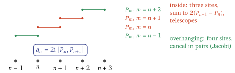
Only neighbours contribute. By (10.2), $\comm{H}{Q_3}=\ii J\sum_{m,n}\comm{P_m}{\comm{P_n}{P_{n+1}}}$. The bond $m$ commutes with $P_n$ and $P_{n+1}$ unless it touches one of the sites $n$, $n+1$, $n+2$, that is unless $m\in\{n-1,n,n+1,n+2\}$ (four distinct bonds, since $N\ge4$). The sum splits into two kinds of term (Figure A.5).

Three-site terms, $m=n$ and $m=n+1$. Write $a=P_n$, $b=P_{n+1}$. Using $a^{2}=b^{2}=1$, $$\comm{a}{\comm{a}{b}}=2b-2aba,\qquad \comm{b}{\comm{a}{b}}=2bab-2a,$$ and by the braid relation $aba=bab$ the sum is $2(b-a)=2(P_{n+1}-P_n)$. Summed over $n$ round the ring, it telescopes to zero.

Four-site terms, $m=n-1$ and $m=n+2$. Relabelling $n\to n+1$ in the first, $$\sum_n\Big(\comm{P_{n-1}}{\comm{P_n}{P_{n+1}}}+\comm{P_{n+2}}{\comm{P_n}{P_{n+1}}}\Big) =\sum_n\Big(\comm{a}{\comm{b}{c}}+\comm{c}{\comm{a}{b}}\Big),$$ now with $a=P_n$, $b=P_{n+1}$, $c=P_{n+2}$. The Jacobi identity says $\comm{a}{\comm{b}{c}}+\comm{c}{\comm{a}{b}}=-\comm{b}{\comm{c}{a}}$, and $\comm{c}{a}=0$ because the bonds $n$ and $n+2$ are disjoint. So $\comm{H}{Q_3}=0$.

$Q_3$ is not a polynomial in $H$. Let $R$ be the reflection of the ring, site $n\mapsto N+1-n$. It maps each bond to a bond, so $RHR^{-1}=H$, and hence $Rf(H)R^{-1}=f(H)$ for every polynomial $f$. It maps $(\boldsymbol\sigma_n\times\boldsymbol\sigma_{n+1})\cdot\boldsymbol\sigma_{n+2}$ to the same triple product of three consecutive sites taken in the reverse order, which is minus it (the three factors act on different sites and commute, and the triple product is antisymmetric in its outer two vectors). So $RQ_3R^{-1}=-Q_3$. Finally $Q_3\ne0$ for $N\ge4$: its terms are Pauli strings on different triples of sites and cannot cancel.

A search for local charges. Every local charge of range at most $3$ is a combination of the translation sums of the $4^{3}=64$ Pauli strings on three sites; for $N\ge5$ they span $49$ dimensions (Proposition 19.2; on smaller rings wrap-around makes some coincide). Requiring $\comm{H}{Q}=0$ is a linear condition on the coefficients, solved by computer. At $N=8$ and $9$ (scripts/check-l13-algebra.py) the solutions are: for XXX exactly $1$, $S^{x}$, $S^{y}$, $S^{z}$, $H$ and $Q_3$; for the $J_1$–$J_2$ chain at $J_2=0.3$, $0.5$ and $0.7$ the same list without $Q_3$; for XXZ at $\XXZ=0.55$, $1$, $S^{z}$, $H$ and an anisotropic cousin of $Q_3$; for XXZ with $J_2$, only $1$, $S^{z}$, $H$. That is a search at two sizes, not a proof about any other.

The ratio for uncorrelated levels. Take two consecutive spacings of Poisson levels, independent with density $e^{-s}$. Then $\tilde r=s_n/s_{n+1}$ has distribution $$\Pr(\tilde r\le x)=\int_0^{\infty}\!\!e^{-t}\,(1-e^{-xt})\,\dd t =1-\frac1{1+x},\qquad\text{density }\frac{1}{(1+x)^{2}} .$$ The density is unchanged by $x\mapsto1/x$ (with its Jacobian), so $r=\min(\tilde r,1/\tilde r)$ has density $2/(1+r)^{2}$ on $[0,1]$, and $$\langle r\rangle_{\mathrm P}=\int_0^{1}\frac{2r}{(1+r)^{2}}\,\dd r =2\Big[\ln(1+r)+\frac{1}{1+r}\Big]_0^{1}=2\ln2-1 .$$ The same computation with the three-level GOE density in place of the exponentials gives $4-2\sqrt3$ (Atas et al.). The check script confirms both, and confirms by simulation that the ratio of two independent exponentials has the density above.

Degenerate spectra. If $H$ has degenerate eigenvalues — because of a symmetry, say — the operators commuting with it no longer commute with each other, and one looks instead for a maximal commuting family among them. Any such family, simultaneously diagonalised, still consists of the linear combinations of $D$ projectors, and the objections of §A.2 return. Von Neumann showed that any commuting family of Hermitian matrices consists of functions of a single one of them (cited by Caux and Mossel) cited.

Which ensemble. The momentum blocks of §A.4 are complex Hermitian, which would suggest the $s^{2}$ repulsion of the unitary ensemble. But reflection combined with complex conjugation maps each block to itself, and that antiunitary symmetry, squaring to $+1$, makes the real, orthogonal ensemble the right reference — which is what Figure A.2 shows. In general $P(s)$ vanishes like $s$, $s^{2}$ or $s^{4}$ — Dyson’s index $1$, $2$ or $4$ — for the orthogonal (an antiunitary symmetry squaring to $+1$), unitary (none) and symplectic (one squaring to $-1$) ensembles. How close the large-matrix law is to the surmise: pooling $3\cdot10^{4}$ bulk spacings of $100$ random $600\times600$ GOE matrices, the fraction below any $s$ differs from the surmise’s by $0.007$ (check-l13-algebra.py, which requires less than $0.015$).

Classes. Caux and Mossel propose a classification by how fast the number of nonzero coefficients of the charges grows with $N$ when they are expanded in a preferred tensor-product basis of operators, such as the Pauli strings ($\sum_nS^{z}_n$ has $N$ of them, although as a matrix it has exponentially many nonzero entries): XXX is “linear”, Haldane–Shastry “quasi-polynomial”, and a generic chain’s conserved operators beyond $1$, $H$ and its symmetries are expected to need exponentially many cited. It is a proposal; this course uses only its moral, which is Proposition 19.2’s.

Berry and Tabor. For an integrable system with $n$ degrees of freedom semiclassical quantisation puts the levels at $E=K(I)$ with the actions on a lattice, $I=\hbar(m+\alpha)$, $m\in\Z^{n}$ (Bohr–Sommerfeld with the Maslov shifts $\alpha$ of Lecture 10’s reading). The levels in a window of energy are the lattice points in a thin shell between two surfaces $K=E$ and $K=E+\delta E$; for $n\ge2$ and a curved, generic $K$, successive lattice points met in energy order come from unrelated parts of the lattice, and Berry and Tabor (1977) argued that their spacings are then Poisson distributed cited. The argument fails where the lattice is seen coherently. For harmonic oscillators $K$ is linear in $I$: with one degree of freedom the levels are equally spaced (a “picket fence”); with commensurate frequencies they are highly degenerate; with incommensurate ones they are neither, and their spacing law depends on the arithmetic of the frequency ratio — but it is not Poisson either (Berry and Tabor treat both cases). The conjecture is for generic integrable systems.

Bohigas, Giannoni and Schmit. For a system whose classical limit is chaotic, the conjecture (1984) is that the spectral fluctuations are those of the random-matrix ensemble with the same antiunitary symmetry: orthogonal with a time reversal squaring to $+1$, unitary without one, symplectic with one squaring to $-1$ cited. Semiclassical arguments through periodic orbits support it; there is no proof.

Spin chains have no classical limit with $N$ fixed, so neither conjecture applies to them as stated; that they nevertheless follow the same pattern is an empirical fact, tested since the early 1990s and on every chain studied in this course, and it is why (P) is a criterion and not a theorem.

Theorem 5.7 describes one regular torus, and Lecture 6 extends its angle coordinates to a neighbourhood. Can the tori over all regular values be given coordinates at once? Not always. The obstruction is called Hamiltonian monodromy; it has nothing to do with the monodromy matrix of Definition 9.1, which shares only the name.

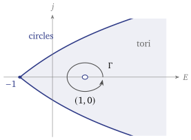
A unit mass on a sphere of unit radius, in unit gravity, with polar angle $\theta$ from the upward vertical, azimuth $\phi$, and $z=\cos\theta$ its height: $$H=\tfrac12p_\theta^{2}+\frac{p_\phi^{2}}{2\sin^{2}\theta}+\cos\theta, \qquad J=p_\phi .$$ $J$, the angular momentum about the vertical, commutes with $H$ by rotational symmetry, and $n=2$. The level sets are compact, since $\abs{p}^{2}\le2(H+1)$. At fixed $J=j$ the height moves in the reduced potential $V_j(z)=j^{2}/2(1-z^{2})+z$, whose minima are the circular conical motions: $j^{2}=-(1-z^{2})^{2}/z$ with energy $E=(3z^{2}-1)/2z$, for $-1<z<0$. These curves bound the image of the energy–momentum map $(H,J)$ (Figure A.6). Over each point of these curves the fibre is a single circle; over their common endpoint $(-1,0)$, the stable equilibrium, it is a point.

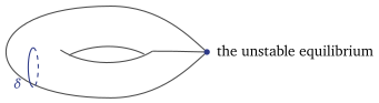
The unstable equilibrium at the top, $z=1$, $p=0$, is the other critical point. There $\dd H=\dd J=0$, it has energy $1$, and its image $(1,0)$ is an isolated critical value in the middle of the image. Every other interior point is a regular value with a compact connected fibre (Cushman–Bates, ch. IV, §3.4), a torus by Theorem 5.7. The fibre over $(1,0)$ contains the equilibrium and the trajectories that leave it and return to it; it is a torus with one cycle pinched to a point (Figure A.7). So the set of regular values is a region with a puncture, and a loop round the puncture cannot be shrunk.

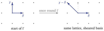
Over each regular value there is a period lattice, and it varies continuously. Choose a basis at one point of the loop $\Gamma$ and carry it continuously round $\Gamma$. It comes back as a basis of the same lattice, so the two differ by an integer matrix of determinant $\pm1$. Take the basis $[\delta],[\gamma]$, with $\delta$ the $J$-orbit and $\gamma$ the cycle made by flowing along $H$ for the first-return time to the same $J$-orbit and then back along that $J$-orbit to the starting point. Then carried once round $\Gamma$, positively oriented, the basis returns as $$\begin{pmatrix}{[\delta]}\\{[\gamma]}\end{pmatrix} \;\longmapsto\; \begin{pmatrix}1&0\\-1&1\end{pmatrix} \begin{pmatrix}{[\delta]}\\{[\gamma]}\end{pmatrix},$$(A.8) (cited: Duistermaat 1980; the matrix, basis and orientation from Cushman–Bates, ch. IV, §5.2). The $J$-cycle comes back to itself — it is defined everywhere by the symmetry — and the other cycle comes back with a copy of it subtracted (Figure A.8). Other sources print $\begin{pmatrix}1&1\\0&1\end{pmatrix}$ for the same system: the entries depend on the basis and the orientation of the loop. The invariant content is that the matrix is a non-trivial shear, and it cannot be undone by any other choice of basis. One way to see it numerically: the rotation number, the advance of $\phi$ in one period of $z$ divided by $2\pi$, continued once round $\Gamma$, comes back changed by exactly $1$.¹

The theorem is about one torus and, via Lecture 6, a neighbourhood of one torus, where the lattice basis can always be chosen continuously. Monodromy is about the whole family: if angle coordinates existed on all the tori over the punctured region at once, the basis they define would be carried round $\Gamma$ unchanged, and (A.8) says it is not. So the spherical pendulum has no global action–angle coordinates (Duistermaat 1980). The same happens round any focus–focus equilibrium: one at which the linearised pair $(H,J)$ is, in suitable canonical coordinates, the pair $(xp_x+yp_y,\ xp_y-yp_x)$ — a hyperbolic scaling and a rotation — provided its critical value is isolated and the nearby fibres, and the singular one, are compact and connected. The top of the sphere is such a point (cited: the geometric monodromy theorem, Cushman–Bates, ch. X, §2). Theorem 5.7 proves the single-torus statement and Lecture 6 the neighbourhood one; global triviality is false.

After quantisation $H$ and $J$ still commute, and their joint eigenvalues $(E,\hbar m)$ form a set of points in the plane. By the Einstein–Brillouin–Keller rule of Lecture 10’s reading, near any regular value the points are the image of the lattice $\hbar(n+\tfrac12,m)$ (a libration in the polar angle, a rotation in the azimuth) under the smooth map $(I_1,I_2)\mapsto(E,J)$ inverse to the action map, asymptotically as $\hbar\to0$: locally a deformed square lattice. Carry a unit cell of it round the critical value $(1,0)$ and it comes back sheared: the quantum numbers label the actions, which pair with the cycles, so the cell’s edges transform contragrediently to (A.8) — in the conventions displayed there by its inverse transpose $\big(\begin{smallmatrix}1&1\\0&1\end{smallmatrix}\big)$, again a non-trivial shear. The joint spectrum has a lattice defect at the puncture, and no choice of two global quantum numbers labels it smoothly (Cushman and Duistermaat 1988) cited. Classical Hamiltonian monodromy — the obstruction to global action–angle variables — is thus visible in a quantum spectrum.

Sources. R. H. Cushman and L. M. Bates, Global Aspects of Classical Integrable Systems, ch. IV (the spherical pendulum: §3.4 the fibres, §5 monodromy) and ch. X; J. J. Duistermaat, “On global action-angle coordinates”, Comm. Pure Appl. Math. 33 (1980); R. H. Cushman and J. J. Duistermaat, “The quantum mechanical spherical pendulum”, Bull. Amer. Math. Soc. 19 (1988).

Integrable systems are exceptional (Lecture 7), so why study them? Because there are two roads from nature to a prediction, and each charges a toll (Figure A.9).

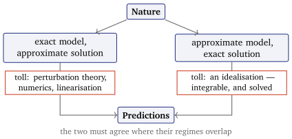
On the left, one writes down the model one believes and solves it approximately: perturbation theory about something simple, numerics, linearisation about a minimum. On the right, one replaces the model by an idealisation that can be solved exactly, and pays in the model instead. A truncation you can solve is worth as much as a truth you cannot, and it is worth more when it is the organising centre of the truth. The harmonic oscillator organises vibrational spectroscopy, and the hydrogen atom organises chemistry, in exactly this way: nobody believes a molecule is a set of oscillators, but every real spectrum is read as a perturbation of that one. Integrable models are the next such centres: exactly solvable, genuinely interacting, and the points from which nearby systems can be studied as perturbations. How far that works is a real question. Lecture 7 answers it classically (the KAM theorem, Theorem 7.8: most of the tori survive a small perturbation, under hypotheses stated there), and Lecture 20 says what is known for a nearly integrable quantum gas (Remark 20.2).

Lecture 7 also adds the caveat that keeps this honest. Integrability is a property of the whole system, not of an approximation to it: truncating the integrable Toda potential at cubic order gives Hénon–Heiles, which is not integrable (Figure 7.5). The right-hand road does not mean “simplify until solvable”; it means finding the exceptional systems exactly as they are, and treating the rest of the world as their perturbation. Nor are the exceptional systems common: in a one-parameter family of potentials that contains Hénon–Heiles, the integrable members are isolated values of the parameter, for conserved quantities of a precise kind (Lecture 7’s reading, which states exactly that much and no more).