Lecture 14
The quantum inverse scattering method, and its classical limit
Course map: G2 and G5, P2 quantised. Lecture 10 solved the Heisenberg chain by a guess and left the question of why it is solvable. This lecture answers with Lecture 9’s three moves, quantised. The chain’s Lax operator satisfies an relation with Yang’s -matrix of Lecture 13, the monodromy satisfies , and the transfer matrices commute at all values of the spectral parameter. Then the lecture restores in the quantum Toda chain and recovers Lecture 9’s -matrix as , sign for sign.
14.1 The question
Lecture 9 made the Toda ring’s integrals commute with one identity for one site; Lecture 10 solved the Heisenberg chain by a guess. So the question is
why do the Heisenberg chain’s charges commute, and what classical structure is this the quantisation of?
The answer: Lecture 9’s structure, with commutators for brackets and Yang’s for (Theorems 14.1 to 14.3); and the classical limit of the quantum Toda chain proves that the dictionary is right (Corollary 14.6). The worked example is the Heisenberg chain’s Lax operator.
14.2 From brackets to commutators
Lecture 9’s site matrices obey the quadratic bracket (9.9); it composes along an ultralocal chain (Theorem 9.7), and its trace makes the transfer matrices Poisson-commute (Corollary 9.8). Quantisation makes the entries of operators and brackets commutators, , and the legs of Definition 9.2 survive. The quantum relation for the monodromy is the relation (14.1) At order it returns (9.9); with the other order of the monodromies it would return , so the order is forced (§14.6). Other books use the other order, each with its own and Lax operator: convert all three together, never one alone. Until §14.6, , and the auxiliary copies of are and , apart from the sites .
14.3 The Lax operator of the Heisenberg chain
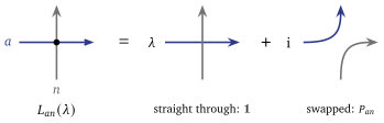
The quantum space is the Heisenberg chain of Lecture 10, , one spin per site. The auxiliary space is one more . The Lax operator at site is (14.2) with the permutation of the auxiliary space with site (Definition 9.4), and . The middle form uses , the identity behind the Hamiltonian (10.2); the matrix is in the auxiliary space, with entries operators on site . Like the Toda site matrix it is linear in the spectral parameter and acts on one site.
Figure 14.1 draws it. Each space is a line: the auxiliary space horizontal, the site vertical. An operator on both is a vertex where they cross, and (14.2) says what happens there: with weight the two states go straight through, and with weight they swap lines, the of Definition 9.4.
Two auxiliary spaces , and one site make three copies of , and on them the only operators needed are the three transpositions , , . Their products are permutations of three objects, and a product of two different transpositions is a -cycle, of which there are two: (14.3) (Follow a vector through each product; this is the computation of Proposition 13.4.)
Theorem 14.1 (The RLL relation). With , (14.4) for all . With in place of it fails.
Proof. Take with a sign and compute the difference of the two sides. It has two parts. The first is , and in everything cancels except the products of two ’s: . The second is the terms having cancelled. By (14.3) the first bracket is , the second , and the triple products are both , so they cancel. The second part is therefore , and This vanishes for and is not zero for , since .
The whole relation is a statement about the permutations of three objects (the check script confirms the residual symbolically).
14.4 From one site to the chain
The monodromy matrix
The monodromy matrix of the chain is the ordered product of the Lax operators along it, (14.5) an operator on : in the auxiliary space a matrix whose entries are operators on the whole chain. As a picture it is a row: one auxiliary line crossing every site in turn (Figure 14.2), Figure 9.1 with operators at the vertices. Operators on different sites commute, so commutes with for : they act on disjoint sets of spaces. That is the quantum form of ultralocality, and it is all the next proof uses.
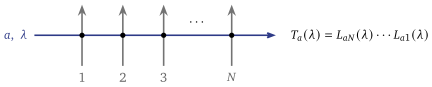
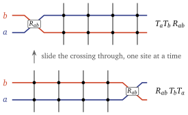
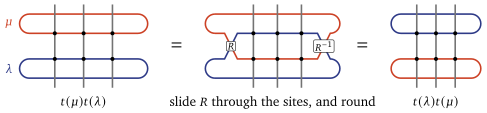
Proof. In , move each to the left past , with which it commutes. The factors pair up by site: Now enters on the left. By (14.4) at site , : it has passed the first pair and reversed it. The same step at each site in turn carries to the right end, leaving , and undoing the pairing gives .
This is the train argument (Figure 14.3): the crossing of the two auxiliary lines is pushed through the row one site at a time, as the bracket was pushed through the product by Leibniz’s rule in Theorem 9.7.
The Lax operator is an -matrix, and RLL is the Yang–Baxter equation
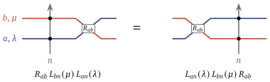
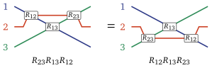
Compare (14.2) with : (14.7) The Lax operator is the -matrix itself, with the site as its second space. It is not : the two differ by . Substitute (14.7) into (14.4); the two minus signs cancel, Rename , , , and put , , so that . Since this is (14.8) the Yang–Baxter equation in its standard form. With , and it is the equation (13.6) that Theorem 13.3 derived from three-body consistency, for the matrix of the delta bosons (13.3). So Theorem 14.1 and Proposition 13.4 are one fact, read twice. In Lecture 13 the three lines were three particles and a two-body collision; in the Heisenberg chain one of the three lines is a site. The fermions of Lecture 13 scatter with , the Lax operator itself.
Figure 14.5 shows the equation as a picture. It is Figure 13.1, and Figure 14.4 is its special case with one line vertical.
14.5 Commuting transfer matrices
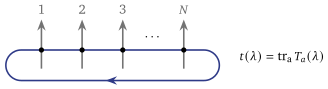
The transfer matrix is the trace of the monodromy over the auxiliary space, (14.9) an operator on the chain alone: in the picture the auxiliary line is closed into a loop (Figure 14.6). It is a polynomial of degree in with operator coefficients, and leading term .
Theorem 14.3 (Commuting transfer matrices). for all .
Proof. , so is invertible for . For such , multiply (14.6) on the left by : . Take the trace over both auxiliary spaces. On the left, , because and have their auxiliary legs in different spaces. On the right, acts on the auxiliary spaces only, as a numerical matrix, and the partial trace is cyclic for such a factor; so . Both sides are polynomials in , so the identity extends to .
This is Corollary 9.8: there the trace of a commutator vanished, here the trace of a conjugate is the trace (Figure 14.7). The coefficients of commute with one another. Whether the family contains a Hamiltonian worth having, and whether its members are local, is the business of Lecture 15.
What gives, and what it does not
The proof used (14.6) and the invertibility of , and not the Yang–Baxter equation. The equation does two other jobs. It supplies Lax operators: by (14.7) the rational , read with a site as its second space, is a Lax operator for its own relation, which is why the Heisenberg chain has one. And it is sufficient, not forced, for the consistency of the relations taken as the definition of an algebra (the readings at the end). Finally, integrability does not require : the free-fermion charges of the Ising chain (Lecture 18) are constructed directly.
14.6 The classical limit, verified: the quantum Toda chain
The Heisenberg chain has no classical limit worth the name — a spin has no small parameter. To test the correspondence of §14.2, quantise Lecture 9’s chain. Restore . The periodic Toda chain has canonical pairs with , represented by on functions of . Keep the site matrix of (9.2) as it stands, (14.10) now with operator entries. No ordering question arises: each entry involves or , never both.
Theorem 14.4 (Quantum Toda: RLL). The site matrix (14.10) satisfies exactly, to all orders in , and fails with . Consequently the monodromy satisfies , and .
Proof. Write with . In the leg notation the entry of is , and of it is the same product in the other order. So their difference is the matrix of commutators , which do not depend on . The only non-zero ones are , exactly times the Poisson brackets used in the proof of Proposition 9.9; that proof computed the whole matrix of brackets, so Next, (conjugating by exchanges the legs), and expanding gives ; the terms, in the same order on both sides, cancel. With the difference of the two sides of the relation is using . It vanishes for only. Sites commute, so Theorem 14.2 and Theorem 14.3 apply verbatim, now with .
The coefficients of are the quantum integrals. They are the expressions of (9.4), now as operators, with no ordering ambiguity since each term has at most one factor per site: , and is the quantum periodic Toda Hamiltonian, a function of the commuting . Its spectral problem was reduced to one-variable quantisation conditions, for small by Gutzwiller (1981) and for all by Sklyanin’s separation of variables (1985) cited.
To compare with Lecture 9, divide by : exactly the of Proposition 9.9, and (14.1)’s expansion with no term. The limit needs a rule for turning operators into functions.
Lemma 14.5 (Symbols). Write an operator polynomial in the ’s with all ’s on the right, , and call , a function of , its symbol. Then
Proof (★). Move each in to the right through ’s functions of by Leibniz’s rule, . The first-order terms of are in the course’s convention.
Corollary 14.6 (The classical limit of ). The symbols of the entries of the quantum monodromy are the entries of the classical monodromy (9.3). At order the relation of Theorem 14.4 becomes Proposition 9.9 and Theorem 9.7, sign for sign.
Proof. Each entry of is a sum of products of entries of different site matrices, which commute, so its symbol is the classical product. Write as and take symbols. On the left the entry is the commutator , whose symbol is by Lemma 14.5: the entry of in Definition 9.2. On the right the symbols of and are both . Divide by and let .
Tracing over both legs, is the order- term of Theorem 14.3. With , false for this chain, the same steps would give : the classical side decides the quantum sign. The check script repeats this computation for two and three sites.
14.7 What it buys
A commuting family for the Heisenberg chain, from one relation for one site (Theorems 14.1 to 14.3). Lecture 15 obtains the chain’s Hamiltonian from its logarithmic derivative and diagonalises the family.
The Yang–Baxter equation, read a second time: the Lax operator is Yang’s with a site as one of its spaces, and is the equation of Lecture 13 (14.8).
G5, closed: the quantum Toda chain’s relation becomes Lecture 9’s quadratic bracket as , sign for sign (Corollary 14.6).
14.8 Caveats, in one place
Status. Theorems 14.1 to 14.4 and Corollary 14.6 are proved; the proof of Lemma 14.5 is a reading. The quantum Toda chain’s spectral problem is cited.
What does not give. It gives commuting operators, not a Hamiltonian worth having or locality (Lecture 15), and not completeness, which stays Lecture 10’s cited question. The independence of the quantum Toda integrals is not shown.
The classical limit is tested on Toda; the Heisenberg chain has no small parameter.
14.9 Two sites by hand
For , , using and . By (14.3), , so and which commutes with itself at any two values, as it must: it involves only . On the triplet , on the singlet . Then , the swap of the two sites, and : Lecture 15 finds the chain’s Hamiltonian in this logarithmic derivative. Repeat for and check that .
14.10 The classical Yang–Baxter equation
The linear Sklyanin bracket (9.11) of Lecture 9’s readings is an assumption about a Poisson bracket, so it must be consistent with the Jacobi identity. Working out what that requires produces the classical form of Lecture 13’s equation.
Put three legs in play, , write for in leg at spectral parameter , and abbreviate . Two facts do the work: when , because they act on disjoint legs; and , which Remark 9.13 showed to be sufficient for antisymmetry of the Poisson bracket but which the bracket does not by itself force. It is therefore a hypothesis of Theorem 14.7, not a consequence of Definition 9.12, and is assumed from here on.
Proof. Since is numerical it passes through a Poisson bracket, so Use and the matrix Jacobi identity in the form on each of the two terms. The first gives and the second the same with , . Now add the two cyclic permutations of this, replacing by as (9.12) allows. The six leftover double commutators pair up, again by matrix Jacobi: for instance Now collect. The first group contributes each double commutator of ’s twice, once from each of the two cyclic terms that produce it, and the two contributions carry different pairs of : so their totals are , and respectively. The three surviving pairs of double commutators, computed as displayed above, contribute exactly , and , which remove the one doubled term in each line. All three are left with , and that is (14.11).
Remark 14.8 (Machine-checked). The collection above is exactly the kind of bookkeeping in which a sign is lost. It is verified in scripts/check-l8-algebra.py, for , with three explicit legs and symbolic entries throughout — sixty free parameters, so the result is an identity and not a sample. The Jacobi sum equals , and — the point of Remark 14.9 — is not identically zero on its own.
Remark 14.9 (Jacobi does not force the CYBE, and saying so matters). Theorem 14.7 gives (14.11), and (14.12) is sufficient for it, not implied by it: the Jacobi identity only requires the triple sum to commute with , and for a particular that is a weaker demand. What makes (14.12) the right thing to impose is that it mentions no at all. One solution then serves every model whose Lax matrix it fits, which is why the classification of -matrices is a subject and the classification of integrable models is not.
One variant deserves its name in passing. Replacing the zero on the right of (14.12) by a specific -independent term gives the modified classical Yang–Baxter equation, whose solutions generate the same structures over a slightly larger class of Lie algebras. Its theory belongs to Lie-bialgebra and Poisson–Lie theory, which this course does not enter; it is named here so that meeting the phrase elsewhere is not a surprise.
The rational solution
Proposition 14.10 (The rational -matrix). satisfies the CYBE (14.12) for every constant .
Proof. Write . The permutation operators satisfy and — both are the two ways of cycling three legs. Calling the difference of those two products , all three commutators are : So the left of (14.12) is because identically.
The cancellation is a statement about the three spectral parameters and nothing else, which is why is free: the normalisation of is fixed by the Lax matrix it is paired with, not by the CYBE. Lecture 9 fixes it for the periodic Toda chain, in (9.10); the open chain of Lecture 9’s readings needs a different, constant .
Two further families solve (14.12): the trigonometric -matrices, in which is replaced by or and the permutation is deformed, and the elliptic ones, built from Weierstrass functions. Belavin and Drinfeld classified the solutions under hypotheses this course has not set up: for valued in with a finite-dimensional simple Lie algebra, in difference form, and non-degenerate in their technical sense (the residue at the simple pole is proportional to the Casimir of an invariant form), every solution is equivalent to a rational, trigonometric or elliptic one cited, and the three degenerate into one another in limits. Those hypotheses are doing real work — dropped, the statement is false, and already fails for , where every commutator in (14.12) vanishes and any function of with a simple pole at the origin solves it. The same trichotomy reappears in the Calogero–Moser potentials (optional lecture B) and in the quantum chains XXX, XXZ and XYZ — it is the same list every time, which is not a coincidence.
The open chain’s is not a solution
The open chain’s constant of (9.22) (Lecture 9’s readings) is skew, , which is (9.12) for a constant ; so Theorem 14.7 applies to it. Does it solve the classical Yang–Baxter equation (14.12)? No. Its left-hand side is (14.13) This identity is cited, not proved here: Babelon–Bernard–Talon, eq. (4.32), state it in operator form, and scripts/check-l9-algebra.py checks it symbolically for . An equation of this shape, with a fixed non-zero right-hand side in place of the zero, is the modified CYBE named above.
And yet the Jacobi identity holds, as it must: the bracket is the canonical one on . Theorem 14.7 asks only that the left of (14.13) commute with , and it does, for every matrix : commutes with (it only swaps them) and with (another leg), so it commutes with the sum, and so does , and so does their commutator. This is Remark 14.9 in a real model: the CYBE is sufficient for Jacobi, and the Toda chain satisfies Jacobi without it.
How unique is ? Adding changes nothing in (9.21), since both commute with ( only swaps the two legs). Babelon–Bernard–Talon, §4.7, derive (9.22) rather than check it, and show it is the only skew constant solution; scripts/check-rmatrix.py (V8) finds, at sampled points for , no constant solutions beyond . Of these, the skew one is itself, which fails the CYBE, while do solve the CYBE (Babelon–Bernard–Talon, (4.33); checked for ) and are not skew, so Theorem 14.7 as proved does not cover them. So no constant for the open chain is both skew and a solution of the CYBE: the route “skew plus CYBE, hence Jacobi” is closed here, and Jacobi holds by the weaker condition above. That is not a defect of the model; it is why Lie-bialgebra theory has a modified equation.
14.11 Reordering three monodromies
Three auxiliary spaces at parameters give three relations (14.6), one for each pair, with .
Proposition 14.11 (Reordering three monodromies). Let satisfy (14.6) with an invertible . Reversing one neighbouring pair at a time gives, along the two possible routes, Hence commutes with every .
Proof. Write (14.6) as for . Route A exchanges the pairs , then , then : , each commuting with the monodromy it does not touch. Route B exchanges , , and gives in the same way. Equating the two results gives the statement.
For a model that satisfies this is automatic — the two routes rewrite one operator. It matters when is taken as the definition of an algebra generated by the entries of , as a Sklyanin bracket can be posited (Lecture 9’s readings): then the two routes yield the commutation condition of the proposition among the generators, and makes it automatic. That is sufficient, not necessary: for , which fails the Yang–Baxter equation, and the condition is again automatic (the check script). It is Remark 14.9 quantised: there the Jacobi identity required a combination of ’s only to commute with , here the associativity of the products requires only to commute with the triple products, and for a particular model that is a weaker demand. What makes the Yang–Baxter equation the right thing to impose is, again, that it mentions no model. (The recipe of (14.7) used ; for a solution without that symmetry it is .) For the Heisenberg chain nothing is left to choose: the check script finds that (14.4) fixes up to a scalar for one and two sites, at generic .
14.12 The Yang–Baxter equation at order , and more
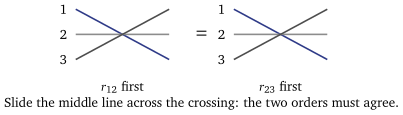
YBE CYBE. Give each line a parameter and write , so (14.8) is . Suppose , in difference form. The terms of order are on both sides. Those of order containing are also the same on both sides; the rest are times the products of two ’s in the order of the factors, so the difference of the two sides at order is a solution of the Yang–Baxter equation has a classical that solves the CYBE (14.12), in the per-leg form of §14.10. For , normalised by (which does not change (14.8), the scalars being the same three on both sides), is Proposition 14.10 at . This is the picture Figure 14.8 promised: the classical slide is the first correction to the quantum one proved; the check script repeats it with generic matrices.
The quantum determinant. At , is times the projector onto the antisymmetric part of , and says that maps the antisymmetric line to itself. The operator by which it multiplies that line (central; for XXX a number) is the quantum determinant, the counterpart of for Toda (9.3). It commutes with every entry of (Korepin, Bogoliubov and Izergin, §VII.8, in their conventions). For the universal algebra defined by on a normalised formal series , the Yangian , the coefficients of the quantum determinant generate the centre (Molev, ch. 1) cited; a spin chain gives a representation of it. For the Heisenberg chain it is the number (the check script, ). Lecture 15 meets its two factors as the eigenvalues of and on the reference state.
Other spins. For a spin at each site, satisfies (14.4) with the same , by a verification that uses only the commutation relations of cited: Korepin, Bogoliubov and Izergin, §VIII.4, (4.6)–(4.8), in their conventions; the check script verifies . The transfer matrix still commutes with itself; but the regular point is lost, since is no longer a permutation, and a local Hamiltonian needs a transfer matrix with a spin- auxiliary space (fusion: Kulish, Reshetikhin and Sklyanin 1981; not treated here).
14.13 Why the zero-curvature equation is not what is quantised
Lecture 8’s and Lecture 9’s readings derived the conservation of from the zero-curvature equation (8.23), , and Lecture 9 proved, separately, the Sklyanin bracket. This lecture quantised only the second. The zero-curvature equation is the equation of motion under one Hamiltonian, and in quantum mechanics equations of motion are not postulated: they follow from once is known. What has to be quantised is the kinematics, the brackets, and from them the commuting family and its Hamiltonians follow. The site-by-site transport survives as the monodromy (14.5), and the bracket as . The Heisenberg equation for under is then a consequence, and is Theorem 14.3, not an input. That is the reason the classical limit of §14.6 was taken in the bracket, not in the equation of motion.
14.14 The Toda pair, quantised
Lecture 12 set the Toda displacement beside Lecture 11’s as a counterpart. For the Toda pair itself the link can be checked. In Proposition 12.1 the relative coordinate and its momentum have , and the relative speed is . Quantised, With and , the solution that decays under the wall is , the modified Bessel function: the chain rule turns this equation into Bessel’s. Far from the wall, , the small-argument form of gives cited: DLMF §§10.25–10.27 an incoming wave , reflected with the phase . Since , the stationary-phase argument of §11.3 puts the incoming packet on and the outgoing one on , with and the digamma function: the packet moves as if reflected by a hard wall at . In the language of §11.3, with the momentum difference, the reflected wave’s phase is up to a constant, and : the wall is . Restoring shifts by and replaces by , so by Stirling’s formula, . The classical orbit of Proposition 12.1, , has its effective wall exactly there, and that wall is what displaces each momentum line by . So the classical displacement is the limit of the quantum one (scripts/check-l16-algebra.py checks the Bessel equation, the asymptotic expansion and the effective-wall limit; the stationary-phase step is argued, not checked; Sutherland §4.2 does the same for the whole hyperbolic family) sketched.
Summary
- The Lax operator satisfies with (Theorem 14.1), which is Lecture 13’s Yang–Baxter equation.
- The train (Theorem 14.2): the monodromy satisfies , and (Theorem 14.3).
- The classical limit (Theorem 14.4 and Corollary 14.6): the quantum Toda chain satisfies exactly with , and at order its relation is Lecture 9’s quadratic bracket with .
- Next: Lecture 15 finds the Heisenberg Hamiltonian in and diagonalises the family by the algebraic Bethe ansatz.
References
E. K. Sklyanin, L. A. Takhtajan and L. D. Faddeev, Theor. Math. Phys. 40 (1979) 688 (the method); L. D. Faddeev, How algebraic Bethe ansatz works for integrable model, Les Houches lectures 1995, arXiv:hep-th/9605187, §§1–3; V. E. Korepin, N. M. Bogoliubov and A. G. Izergin, Quantum Inverse Scattering Method and Correlation Functions, Cambridge University Press (1993), §§VI.1–VI.5, §VII.8 (the quantum determinant), §VIII.4 (higher spin); M. C. Gutzwiller, Ann. Phys. 133 (1981) 304 and E. K. Sklyanin, Lect. Notes Phys. 226 (1985) 196 (the quantum Toda chain); A. Molev, Yangians and Classical Lie Algebras, American Mathematical Society (2007), Chapter 1 (the Yangian and its centre); O. Babelon, D. Bernard and M. Talon, Introduction to Classical Integrable Systems, Cambridge University Press (2003), Ch. 2–3 (the classical Yang–Baxter equation) and §4.7 (the open chain’s ). The conventions for the ordering of , of the monodromy and for the sign in differ between these sources; see §14.2.
End of Lecture 14
The quantum inverse scattering method, and its classical limit
Lecture 14 · Contents
Keyboard
- → Space PgDn
- next screen, stopping before an equation, figure or statement it would cut
- ← PgUp
- previous screen
- ↓ ↑ wheel
- scroll freely
- Home End
- the start or the end
- S
- Full ↔ Spine, keeping your place
- T
- Think first on or off
- R
- reveal the next hidden proof
- C
- Core only on or off
- G
- contents: jump to a section or a statement
- + −
- text size
- D
- light or dark
- F
- full screen
- P
- pen on or off: draw on the text
- E
- erase the ink on the screen
- Z double-click
- enlarge an equation, figure or table; Z again for the next
- L
- laser pointer on or off
- B .
- blank the screen
- M
- move the toolbar: right, bottom, left, top
- ?
- this help
- Esc
- close a panel