B.1 The question

The Toda chain of Lecture 8 and Lecture 9 was integrable with neighbours interacting. Let every pair interact, through $g^{2}/(q_j-q_k)^{2}$ . So the question is

why is a gas in which every particle pushes every other integrable, and why does every trapped orbit, and every trapped quantum state, return after the same time?

The answer: the gas is free motion in a space of matrices, seen through its eigenvalues (Theorems B.8 and B.9); quantum mechanically, the trapped Hamiltonian is conjugate to one that is triangular in the degree (Theorem B.16). The worked example is two particles (Example B.4).

B.2 The model, and Moser’s Lax pair

$N$ unit masses on a line, positions $q_1,\dots,q_N$ , interacting in pairs: $H=\frac12\sum_{j=1}^{N}p_j^{2}+g^{2}\sum_{j<k}V(q_j-q_k),\qquad g>0 .$ (B.1) Four even pair potentials make this integrable (drawn in the first reading):

model	$V(x)$	motion
rational	$1/x^{2}$	scattering
hyperbolic	$1/\sinh^{2}x$	scattering, short range
trigonometric	$1/\sin^{2}x$	on a circle, confined
elliptic	$\wp(x)$	on a circle, confined

$\wp$ is Weierstrass’s doubly periodic function (the first reading at the end of this lecture), and the other three are its limits, up to scale and an additive constant, as one or both periods become infinite. The list rational / trigonometric (with hyperbolic) / elliptic is the list of classical $\rmat$ -matrices in Lecture 14’s reading; that it recurs is not a coincidence, but this course does not prove it. Every $V$ has a double pole at $0$ and is repulsive near it, so two particles never meet and keep their (on the circle, cyclic) order. We work with the rational model.

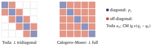
Moser’s Lax matrix fills every off-diagonal slot, one for each pair. With $q_{jk}:=q_j-q_k$ and $x$ a real odd function, $L_{jk}=p_j\,\delta_{jk}+\ii g\,x(q_{jk})\,(1-\delta_{jk}),\qquad M_{jk}=-\ii g\,x'(q_{jk})\ (j\ne k),\qquad M_{jj}=-\ii g\sum_{l\ne j}V(q_{jl}) .$ (B.2) $L$ is Hermitian, since $x$ is odd, and $\tr L^{2}=\sum_jp_j^{2}+g^{2} \sum_{j\ne k}x(q_{jk})^{2}$ , which is $2H$ exactly when $x^{2}=V$ .

Theorem B.1 (Moser’s Lax pair proved in the reading). Let $x(u)$ be $1/u$ , $1/\sin u$ or $1/\sinh u$ , and $V=x^{2}$ . With $L$ and $M$ as in (B.2), $\dot L=\comm{M}{L}$ along every solution of (B.1), for every $N$ .

The elliptic model has a pair of the same kind cited, and Theorem B.9 derives the rational $L$ and $M$ again, from nothing. By Theorem 8.2 the $F_k=\tr L^{k}$ are conserved and real ( $F_1$ the total momentum, $F_2=2H$ ).

Theorem B.2 (Independence proved in the reading). For these $x$ , $F_1,\dots,F_N$ are independent on a dense open set.

Involution is where the model leaves Lecture 9’s method behind.

Proposition B.3 (No numerical $\rmat$ ). For the rational model with $N=2,3$ no constant $\rmat$ satisfies $\pb{\leg{L}{1}}{\leg{L}{2}}=\comm{\leg{\rmat}{12}}{\leg{L}{1}+\leg{L}{2}}$ , nor the weaker two-term form of the reading; for $N=3$ not even an $\rmat$ that depends on the point satisfies the first.

Proof. Each is an inconsistent finite linear system, in exact arithmetic (scripts/check-l11-algebra.py; the points are in the reading).

What exists is the two-term form with an $\rmat$ that depends on the positions cited: Avan and Talon 1993, and the cyclicity argument of Lecture 9’s reading never needed $\rmat$ constant, so the $F_k$ are in involution (the reading). The reduction below says why that had to hold.

B.3 Free motion in disguise

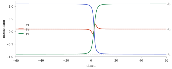
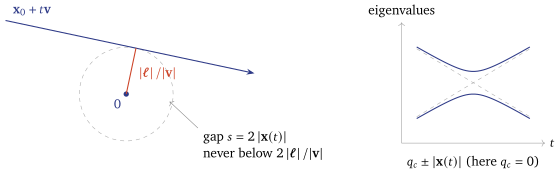
Move two $3\times3$ Hermitian matrices along a straight line, $X(t)=X_0+t\,P_0 .$ (B.3) Nothing could be freer. Yet the three eigenvalues of $X(t)$ , straight lines far in the past and future, do not cross: they approach, slow down and turn away, as if they repelled (Figure B.1). For the right $X_0$ , $P_0$ they obey exactly the rational Calogero–Moser equations.

Figure B.1. The eigenvalues of

X_0+tP_0

(

N=3

,

X_0=\operatorname{diag}(q)

,

P_0

Moser’s

L

at

g=0.6

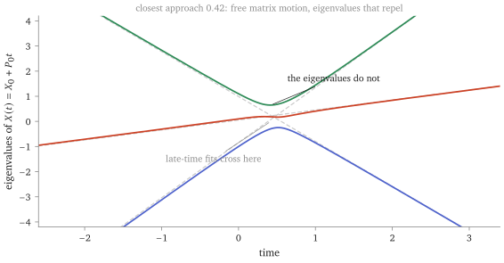
). The dashed lines, late-time straight-line fits, cross; the eigenvalues do not. (scripts/figures/cm_eigenvalue_repulsion.py integrates Calogero–Moser from the same data and asserts agreement to

10^{-7}

.)

Example B.4 (Two eigenvalues and the centrifugal barrier). For $N=2$ every Hermitian matrix is $X=q_c\Id+\mathbf x\cdot\boldsymbol\sigma$ , with $q_c\in\R$ , $\mathbf x\in\R^{3}$ and $\boldsymbol\sigma$ the Pauli matrices. Its eigenvalues are $q_c\pm\abs{\mathbf x}$ , so their gap is $s=2\abs{\mathbf x}$ . Along (B.3), $q_c$ moves uniformly and $\mathbf x(t)=\mathbf x_0+t\mathbf v$ is a free particle in $\R^{3}$ . Its distance from the origin feels the centrifugal barrier: with $\boldsymbol\ell=\mathbf x\times\mathbf v$ conserved, $\abs{\mathbf v}^{2}=\dot r^{2}+\abs{\boldsymbol\ell}^{2}/r^{2}$ , $r=\abs{\mathbf x}$ . In terms of the gap, $\abs{\mathbf v}^{2}=\tfrac14\dot s^{2}+\frac{4\abs{\boldsymbol\ell}^{2}}{s^{2}},$ which is the relative energy of two Calogero–Moser particles, $\tfrac14\dot s^{2}+g^{2}/s^{2}$ , with $g=2\abs{\boldsymbol\ell}$ . The eigenvalues repel because a straight line that misses the origin cannot reach it; they would collide only if $\boldsymbol\ell=0$ .

For $N$ particles the rotations become $\U(N)$ acting on matrices, the angular momentum becomes $\comm{X}{P}$ , and one idea that $N=2$ hides is needed: which value to fix it at.

B.4 A conserved commutator, and a level with no collisions

The phase space is $\Herm(N)\times\Herm(N)$ , points $(X,P)$ (from here on $P$ is a matrix of momenta, not the permutation of Proposition B.3), with the real components of $X$ and $P$ in an orthonormal basis for $\tr(AB)$ canonical, $\symp=\tr(\dd X\wedge\dd P)$ , and $H=\tfrac12\tr P^{2}$ : a free particle in $\R^{N^{2}}$ . Conjugating both matrices by $U\in\U(N)$ is a rotation of $\R^{N^{2}}$ applied to $X$ and to $P$ alike, so symplectic, and leaves $H$ invariant; the conserved quantity it supplies, by Lecture 2’s Noether principle, is $\comm{X}{P}$ , the momentum map of conjugation (the reading). For $N=2$ its traceless part is $2\ii\boldsymbol\ell\cdot\boldsymbol\sigma$ .

Corollary B.5 (Conserved and equivariant).

(a)
$\comm{X}{P}$ is constant along the free flow and along that of the trapped $H=\tfrac12\tr(P^{2}+\freq^{2}X^{2})$ : $\frac{\dd}{\dd t}\comm{X}{P}=\comm{P}{P}+\comm{X}{\dot P}=0$ , since $\dot P$ is $0$ or $-\freq^{2}X$ .
(b)
$\comm{UXU^{\dagger}}{UPU^{\dagger}}=U\comm{X}{P}U^{\dagger}$ .

So $\comm{X}{P}=\xi$ , anti-Hermitian and traceless, is a constraint imposed once and for all. By (b), conjugation carries the level $\xi$ to $U\xi U^{\dagger}$ ; what acts on one level set is the stabiliser $\U(N)_\xi=\{U:U\xi U^{\dagger}=\xi\}$ , the residual gauge group, whose orbits are single physical states. The level we need is $\xi=\ii g\,(ee^{T}-\Id),\qquad e=(1,\dots,1)^{T},\qquad \text{that is}\quad \xi_{jk}=\ii g(1-\delta_{jk}),\quad g>0 .$ (B.4)

Proposition B.6 (The stabiliser of $\xi$ ). $U\in\U(N)_\xi$ if and only if $Ue=e^{\ii\theta}e$ for some $\theta$ , since $U\xi U^{\dagger}=\ii g(Ue\,(Ue)^{\dagger}-\Id)$ .

Lemma B.7 (No collisions). Let $\comm{X}{P}=\xi$ , and diagonalise, $X=VQV^{\dagger}$ . Then $w=V^{\dagger}e$ has $\abs{w_j}=1$ for every $j$ , and $X$ is regular: its eigenvalues are distinct.

Proof. Conjugating by $V^{\dagger}$ , $\comm{Q}{\tilde P}=\ii g(ww^{\dagger}-\Id)$ with $\tilde P=V^{\dagger}PV$ . Entry by entry, $\comm{Q}{\tilde P}_{jk}=(q_j-q_k)\tilde P_{jk}$ . On the diagonal the left side is $0$ , so $\ii g(\abs{w_j}^{2}-1)=0$ . Off the diagonal, $(q_j-q_k)\tilde P_{jk}=\ii g\,w_j\bar w_k$ , whose right side has modulus $g\ne0$ ; so $q_j\ne q_k$ .

This is Figure B.1 in one line: on the level set of $\xi$ the eigenvalues of $X$ never meet.

B.5 The reduction: Moser’s $L$ is the free momentum

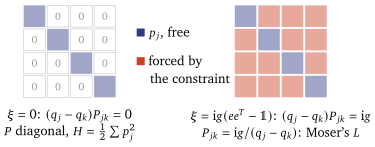
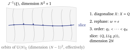
The recipe: bring $X$ to a normal form with the residual gauge group (gauge fixing), solve the constraint for what is left of $P$ , and read off $H$ . At $\xi=0$ it returns free particles, the wrong model (the reading). At (B.4):

Theorem B.8 (Calogero–Moser by reduction (Kazhdan–Kostant–Sternberg)).

(a)
Every point of the level set $\{\comm{X}{P}=\xi\}$ is $\U(N)_\xi$ -equivalent to exactly one point of the slice $X=Q=\operatorname{diag}(q_1,\dots,q_N),\quad q_1<\dots<q_N,\qquad P=L(q,p),\quad L_{jk}=p_j\delta_{jk}+\frac{\ii g\,(1-\delta_{jk})}{q_j-q_k},$ (B.5) which is Moser’s $L$ of (B.2) with $x=1/u$ .
(b)
On the slice, $H=\tfrac12\tr L^{2}=\tfrac12\sum_jp_j^{2} +g^{2}\sum_{j<k}(q_j-q_k)^{-2}$ , the rational Calogero–Moser Hamiltonian.
(c)
The reduced phase space is the chamber $q_1<\dots<q_N$ times $\R^{N}$ , with its canonical form $\sum_j\dd q_j\wedge\dd p_j$ proved in the reading, from the cited Marsden–Weinstein theorem.

Proof. (a) Take $(X,P)$ with $\comm{X}{P}=\xi$ and diagonalise, $X=VQV^{\dagger}$ , eigenvalues increasing. By Lemma B.7, $w=V^{\dagger}e$ has entries of modulus one, so $D=\operatorname{diag}(w_1,\dots,w_N)$ is unitary. Put $U=VD$ . Then $U^{\dagger}XU=D^{\dagger}QD=Q$ , and $U^{\dagger}e=D^{\dagger}w=e$ , so $U\in\U(N)_\xi$ by Proposition B.6. The pair $(Q,L)=(U^{\dagger}XU,U^{\dagger}PU)$ still satisfies $\comm{Q}{L}=U^{\dagger}\xi U=\xi$ , that is $(q_j-q_k)L_{jk}=\ii g$ for $j\ne k$ ; so $L_{jk}=\ii g/(q_j-q_k)$ , and the diagonal $p_j:=L_{jj}$ is free. Uniqueness: a $U\in\U(N)_\xi$ carrying one slice point to another fixes the ordered $Q$ , so maps each eigenline of $Q$ to itself and is diagonal; with $Ue=e^{\ii\theta}e$ it is the scalar $e^{\ii\theta}\Id$ , which moves nothing. (b) $L_{jk}L_{kj}=\ii g\cdot\ii g/\big((q_j-q_k)(q_k-q_j)\big)=g^{2}/(q_j-q_k)^{2}$ .

Theorem B.9 (The eigenvalues of free matrix motion). Let $(q(t),p(t))$ be the rational Calogero–Moser trajectory from $(q(0),p(0))$ , $q_1(0)<\dots<q_N(0)$ . Then:

(a)
$q_1(t)<\dots<q_N(t)$ are the eigenvalues of $X(t)=Q(0)+t\,L(0),\qquad L(0)=L(q(0),p(0)),$ (B.6) for all $t\in\R$ , and in particular the flow is complete;
(b)
$L(t)=L(q(t),p(t))$ equals $U^{\dagger}L(0)U$ for a smooth unitary gauge $U(t)\in\U(N)_\xi$ , $U(0)=\Id$ , with $U^{\dagger}X(t)U=\operatorname{diag}(q(t))$ , and $\dot L=\comm{M}{L}$ with $M=-U^{\dagger}\dot U,\qquad M_{jk}=\frac{\ii g}{(q_j-q_k)^{2}}\ (j\ne k),\qquad M_{jj}=-\ii g\sum_{l\ne j}\frac{1}{(q_j-q_l)^{2}},$ (B.7) which is Moser’s $M$ of (B.2) for $x=1/u$ .

Proof sketched; in full in the reading. Run the argument backwards. The free motion (B.6) stays on the level $\xi$ (Corollary B.5), so its eigenvalues never meet (Lemma B.7) and the gauge of Theorem B.8(a) can be chosen smoothly in $t$ : the columns of $U(t)$ are the eigenprojections of $X(t)$ applied to $e$ . Differentiating $U^{\dagger}XU$ gives $\dot{\tilde q}_j=\tilde p_j$ on the diagonal and fixes the off-diagonal of $A=U^{\dagger}\dot U$ ; the condition $U^{\dagger}e=e$ fixes its diagonal (every row of $A$ sums to zero); so $M=-A$ is (B.7), and the diagonal of $\dot{\tilde L}=\comm{M}{\tilde L}$ is Newton’s law $\dot{\tilde p}_j=2g^{2}\sum_{l\ne j}(\tilde q_j-\tilde q_l)^{-3}$ . The eigenvalues therefore solve Calogero–Moser from the right initial data, and uniqueness of solutions (Theorem 1.5) finishes it.

Moser’s $L$ is the free momentum $P$ in the gauge where $X$ is diagonal, so isospectrality is the conservation of $P$ ; Moser’s $M$ is minus the velocity of that gauge. The $\tr L^{k}=\tr P^{k}$ are functions of $P$ alone, which Poisson-commute trivially on $\Herm(N)^{2}$ , and the Marsden–Weinstein theorem passes brackets of invariant functions to the reduced space: involution is automatic.

Scattering. For large $\abs t$ , (B.6) has eigenvalues $t\lambda_k+\beta_k+O(1/t)$ , with the same offsets $\beta_k$ as $t\to\pm\infty$ : momenta permuted and nothing displaced, unlike Lecture 12’s Toda lines (Proposition 12.1; the reading has the details).

The trap. Replace $H$ by $\tfrac12\tr(P^{2}+\freq^{2}X^{2})$ , which on the slice is the rational model plus $\tfrac12\freq^{2}\sum_jq_j^{2}$ . It is still $\U(N)$ -invariant, $\comm{X}{P}$ is still conserved, the matrix now oscillates, $\dot X=P$ , $\dot P=-\freq^{2}X$ , and the same proof, with one extra term $-\freq^{2}\tilde q_j$ in $\dot{\tilde p}_j$ , gives:

Corollary B.10 (The trap). The trapped rational Calogero–Moser positions are the eigenvalues of $Q(0)\cos\freq t+\freq^{-1}L(0)\sin\freq t$ . Every orbit returns to its starting point at $t=2\pi/\freq$ .

B.6 The quantum gas, and its Jastrow ground state

Quantise the trapped rational model, in units $\hbar=m=1$ (so the classical Hamiltonian above is the literal classical limit; not the $\hbar=2m=1$ of Lecture 11’s gas): $H_{\mathrm C}=-\frac12\sum_{j=1}^{N}\partial_j^{2} +\sum_{i<j}\frac{\beta(\beta-1)}{(x_i-x_j)^{2}} +\frac{\freq^{2}}2\sum_{j=1}^{N}x_j^{2},\qquad \beta\ge\tfrac12 .$ (B.8) With $\hbar$ restored the coupling is $\hbar^{2}\beta(\beta-1)$ , and $\hbar\beta\to g$ as $\hbar\to0$ . The model is the bosonic Friedrichs extension from functions supported away from every collision, whose eigenfunctions vanish there like $\abs{x_i-x_j}^{\beta}$ , the larger of the two possible powers cited: Reed and Simon II, §X.1; the reading says when this is a choice. On the chamber $x_1<\dots<x_N$ , $\Delta=\prod_{i<j}(x_j-x_i)>0$ .

Theorem B.11 (The Jastrow state proved in the reading). The function $\psi_0^{\mathrm C}=\Delta^{\beta}e^{-\freq\sum_jx_j^{2}/2}$ (B.9) satisfies $H_{\mathrm C}\psi_0^{\mathrm C}=E_0^{\mathrm C}\psi_0^{\mathrm C}$ with $E_0^{\mathrm C}=\freq\Bigl(\frac N2+\frac{\beta N(N-1)}2\Bigr),$ (B.10) and without the trap $H_{\mathrm C}\big|_{\freq=0}\,\Delta^{\beta}=0$ .

The proof is two identities in the logarithmic derivative of $\Delta^{\beta}$ , of which the one that matters is that three-index terms cancel. At $\beta=1$ the state is the Slater determinant of the $N$ lowest oscillator states, and (B.10) is $\freq\sum_{n<N}(n+\tfrac12)$ . It is the ground state of this operator, positive and in its form domain sketched in the reading; positivity alone would not decide it.

B.7 Dunkl operators

Lecture 8 got charges from a Lax matrix, Lecture 14 from a transfer matrix. Here first-order operators commute outright, by carrying a transposition inside them.

Definition B.12 (Dunkl operators). Let $s_{ij}$ exchange the arguments $x_i$ and $x_j$ of a function. For $i=1,\dots,N$ put $D_i=\partial_i+\beta\sum_{j\ne i}\frac{1-s_{ij}}{x_i-x_j} .$ (B.11)

$D_i$ maps polynomials to polynomials, $(1-s_{ij})f$ being divisible by $x_i-x_j$ ; and $s_{ij}$ is an operator, not a number, so $D_i$ is not a derivation (the tutorial computes the failure of Leibniz’s rule).

At $N=2$ the commutativity is the translation invariance of $x_1-x_2$ (the reading); in general:

Theorem B.13 (Commutativity proved in the reading). $\comm{D_i}{D_j}=0$ for all $i,j$ , on polynomials.

The first charge is familiar: the deformation cancels pairwise, and $\sum_iD_i=\sum_i\partial_i$ is $\ii$ times the total momentum. The second is the Hamiltonian. Write $\Lambda^{\mathrm{sym}}$ for the symmetric polynomials.

Theorem B.14 (The symmetric restriction proved in the reading). For $f\in\Lambda^{\mathrm{sym}}$ , $-\frac12\sum_iD_i^{2}f =\Delta^{-\beta}\Bigl(H_{\mathrm C}\big|_{\freq=0}\Bigr)\Delta^{\beta}f =-\frac12\sum_i\partial_i^{2}f -\beta\sum_{i<j}\frac{\partial_if-\partial_jf}{x_i-x_j} .$ (B.12) So $-\tfrac12\sum_iD_i^{2}$ preserves $\Lambda^{\mathrm{sym}}$ and sends its homogeneous component of degree $d$ into degree $d-2$ , possibly to zero.

Corollary B.15 (Commuting charges, with no transfer matrix). The operators $I_k=\sum_iD_i^{k}$ , restricted to $\Lambda^{\mathrm{sym}}$ , preserve it and commute, $\comm{I_k}{I_m}=0$ ; $I_1$ is $\ii$ times the total momentum and $-\tfrac12I_2$ the gauge-transformed Hamiltonian (B.12).

Proof. A permutation relabels derivatives, differences and transpositions together, so each $I_k$ is symmetric and preserves $\Lambda^{\mathrm{sym}}$ ; they commute by Theorem B.13.

B.8 The trapped spectrum, and isochrony

The whole spectrum follows from Theorem B.14 alone. The homogeneous symmetric polynomials of degree $n$ have a basis of monomial symmetric polynomials $m_\kappa$ , one for each partition $\kappa$ of $n$ into at most $N$ parts.

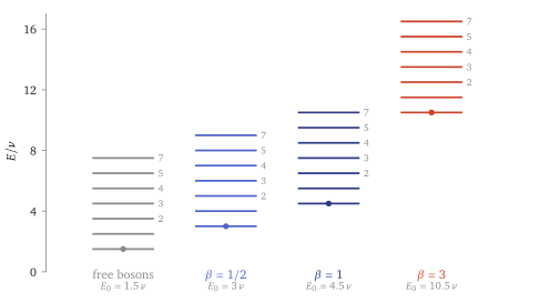
Theorem B.16 (The trapped spectrum). On $\Lambda^{\mathrm{sym}}$ , $\bigl(\psi_0^{\mathrm C}\bigr)^{-1}H_{\mathrm C}\,\psi_0^{\mathrm C} =E_0^{\mathrm C}+\freq\sum_ix_i\partial_i-\frac12\sum_iD_i^{2} .$ (B.13) The eigenvalues of $H_{\mathrm C}$ on $\psi_0^{\mathrm C}\Lambda^{\mathrm{sym}}$ are $E=E_0^{\mathrm C}+\freq n,\qquad n=0,1,2,\dots,$ (B.14) the multiplicity of $E_0^{\mathrm C}+\freq n$ being the number of partitions of $n$ into at most $N$ parts.

Proof. Write $G=e^{-\freq\sum x_j^{2}/2}$ and let $h=\Delta^{\beta}f$ with $f$ symmetric. From $\partial_i^{2}(Gh)=G(\partial_i^{2}h-2\freq x_i\partial_ih-\freq h +\freq^{2}x_i^{2}h)$ , $G^{-1}\Bigl(-\frac12\sum_i\partial_i^{2}+\frac{\freq^{2}}2\sum_ix_i^{2}\Bigr) (Gh) =-\frac12\sum_i\partial_i^{2}h+\freq\sum_ix_i\partial_ih+\frac{\freq N}2h ,$ the trap having cancelled. Adding the pair potential and conjugating by $\Delta^{\beta}$ , the first term becomes $-\tfrac12\sum D_i^{2}f$ by Theorem B.14, while the Euler operator picks up the degree of $\Delta^{\beta}$ : $\Delta^{-\beta}\sum x_i\partial_i(\Delta^{\beta}f) =\sum x_i\partial_if+\tfrac12\beta N(N-1)f$ . The constants assemble into $E_0^{\mathrm C}$ , which is (B.13).

The right side is triangular in the degree: $\sum x_i\partial_i$ multiplies a homogeneous polynomial of degree $d$ by $d$ , and $-\tfrac12\sum D_i^{2}$ lowers the degree by two or annihilates. On the symmetric polynomials of degree at most $d$ the matrix is block-triangular, the block of degree $n$ carrying the scalar $\freq n$ ; different blocks carry different scalars, so there is no Jordan obstruction, and the lower-degree part of each eigenvector is solved for recursively. The eigenvalues are $\freq n$ , $n\le d$ , with multiplicity the dimension of the degree- $n$ block; let $d\to\infty$ . That these are all the eigenvalues is a density statement: the measure $\abs\Delta^{2\beta}e^{-\freq\abs x^{2}}\dd x$ has finite exponential moments, so polynomials are dense in its $L^{2}$ cited.

Remark B.17 (The classical face). Classically every trapped orbit returns after $2\pi/\freq$ (Corollary B.10), whatever its energy. Quantum mechanically $e^{-\ii H_{\mathrm C}t}$ at $t=2\pi/\freq$ is a phase times the identity, so every state returns. Neither is a limit of the other: two theorems in the same role, a type-A row of the Dictionary box.

Isochrony of the trapped model (Corollary B.10)⟶the equally spaced spectrum $E_0+\freq n$ (Theorem B.16): every state returns after $2\pi/\freq$ (type A)

B.9 What it buys

A second road to integrability: not an $\rmat$ -matrix but a reduction — a free system, a symmetry, a constraint, a gauge fixing (Theorem B.8) — in which Moser’s $L$ and $M$ are the free momentum and the gauge velocity, and involution is automatic.
The motion in closed form (Theorem B.9): momenta permuted and nothing displaced; in a trap, one period for every orbit.
A quantum integrable model with no Bethe ansatz and no transfer matrix, whose trapped spectrum is the quantum face of isochrony (Theorem B.16).

B.10 Caveats, in one place

Status. Proved here: Theorem B.8(a),(b) and Theorem B.16 (up to the cited density of polynomials). Sketched here, proved in the readings: Theorem B.9, whence Corollary B.10. Proved in the readings: Theorem B.1, Theorem B.2, Theorem B.11, Theorem B.13, Theorem B.14. Cited: the elliptic pair, the dynamical $\rmat$ , and the Marsden–Weinstein theorem behind Theorem B.8(c) and the involution by reduction. Proposition B.3 is an exact computation.
Only the rational model is reduced here (the others: the readings, cited).
The trapped gas: that it has $N$ independent classical integrals in involution, and $N$ algebraically independent quantum charges, is cited; what is proved is isochrony and the spectrum.
No torus on the line: the untrapped gas has no compact level sets, and scatters (the reading).

B.11 Moser’s Lax pair, derived

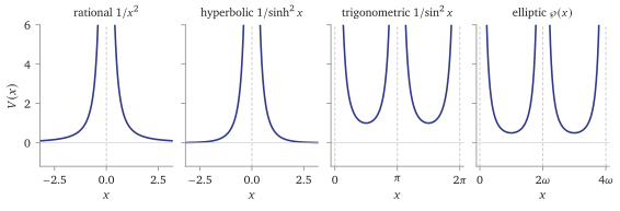
Figure B.2. The four pair potentials, each with a double pole at

x=0

. The first two decay (scattering); the last two are periodic (particles on a circle) (scripts/figures/cm_potentials.py, which samples the leading pole

x^{-2}

at two small

x

, the parity, the period and Weierstrass’s equation).

The Weierstrass function is, for a lattice $\Lambda=2\omega_1\Z+2\omega_2\Z$ in $\C$ — here always rectangular, with $\omega_1$ real and $\omega_2$ purely imaginary, so that $\wp$ is real on the real line with real period $2\omega_1$ — $\wp(x)=\frac1{x^{2}}+\sum_{w\in\Lambda\setminus\{0\}} \Big(\frac1{(x-w)^{2}}-\frac1{w^{2}}\Big),$ even, doubly periodic ( $\wp(x+2\omega_1)=\wp(x+2\omega_2)=\wp(x)$ ), with a double pole at every lattice point. We use nothing else about it. Sending one period to infinity turns it, up to scale and an additive constant, into $1/\sin^{2}$ or $1/\sinh^{2}$ ; sending both gives $1/x^{2}$ (Perelomov, §3.1). The elliptic model contains the other three as limits. Two of the four potentials, the trigonometric and the elliptic, are periodic, with period $d=\pi$ or $2\omega_1$ , so the positions matter only modulo $d$ : $N$ particles on a circle of length $d$ , each hemmed in by its neighbours, confined. The cyclic order of the particles is preserved; in each fixed cyclic order a configuration is a point of the circle (where particle $1$ is) and $N$ positive gaps adding up to $d$ (Perelomov, (3.1.16)), so that component of phase space is a circle times an open $(N-1)$ -simplex, times $\R^{N}$ for the momenta.

Choosing $L$ . Follow Lecture 8’s recipe (§8.4): find $L$ with $\tr L^{2}=2H$ , then solve for $M$ . Every pair interacts, so every off-diagonal slot is used: try

$L_{jk}=p_j\,\delta_{jk}+\ii g\,x(q_j-q_k)\,(1-\delta_{jk}),$ (B.15) with $x$ a real odd function still to be found. Oddness makes $L$ Hermitian, since $L_{kj}=\ii g\,x(q_k-q_j)=-\ii g\,x(q_j-q_k)=\overline{L_{jk}}$ , and then $\tr L^{2}=\sum_jp_j^{2}+\sum_{j\ne k}(\ii g)^{2}x(q_{jk})\,x(q_{kj}) =\sum_jp_j^{2}+g^{2}\sum_{j\ne k}x(q_{jk})^{2}, \qquad q_{jk}:=q_j-q_k .$ Within this ansatz, this is $2H$ exactly when $x^{2}=V$ . So $x=1/u$ for the rational model, and likewise $1/\sin u$ and $1/\sinh u$ (Figure B.3); this is (B.2).

Figure B.3. The shape of the Lax matrix follows the interaction. Toda’s neighbours give a tridiagonal

L

; in Calogero–Moser every pair interacts, and every off-diagonal slot is filled.

Solving for $M$ .

Along the flow, $\dot L_{jj}=\dot p_j$ and, for $j\ne k$ , $\dot L_{jk}=\ii g\,x'(q_{jk})(p_j-p_k)$ . We look for $M$ with $\comm{M}{L}$ equal to this. $M$ is never unique — adding any function of $L$ changes nothing ( $M$ is determined only up to the commutant of $L$ , Lecture 8) — so we make an ansatz, the natural one for a pairwise interaction: $M$ is anti-Hermitian, depends on the positions only, and $M_{jk}$ ( $j\ne k$ ) is a function of $q_j-q_k$ . Within it, three observations fix $M$ .

The part linear in $p$ . Off the diagonal, the only terms of $\comm{M}{L}_{jk}$ containing momenta then come from the diagonal of $L$ : $M_{jk}L_{kk}-L_{jj}M_{jk}=M_{jk}(p_k-p_j)$ . Matching $\dot L_{jk}$ forces $M_{jk}=-\ii g\,x'(q_{jk})\qquad(j\ne k),$ (B.16) anti-Hermitian because $x'$ is even.

The diagonal. $\comm{M}{L}_{jj}$ involves only off-diagonal entries: $\comm{M}{L}_{jj}=\sum_{l\ne j}\big(M_{jl}L_{lj}-L_{jl}M_{lj}\big) =-g^{2}\sum_{l\ne j}2x(q_{jl})x'(q_{jl}) =-g^{2}\sum_{l\ne j}V'(q_{jl})=\dot p_j ,$ using oddness twice and $V'=2xx'$ . So the diagonal of the Lax equation is Newton’s law, whatever the diagonal of $M$ is.

The rest. What remains of $\comm{M}{L}_{jk}$ , $j\ne k$ , must vanish: the terms through a third index $l$ , and the diagonal of $M$ , $(\ii g)^{2}\sum_{l\ne j,k}\big(x(a)x'(b)-x'(a)x(b)\big) +\ii g\,x(a+b)\,(M_{jj}-M_{kk})=0, \qquad a=q_{jl},\ b=q_{lk},\ a+b=q_{jk}.$ This is where the model is decided. Suppose $x$ satisfies the functional identity $x(a)x'(b)-x'(a)x(b)=x(a+b)\big(V(a)-V(b)\big).$ (B.17) Then the condition becomes $M_{jj}-M_{kk}=-\ii g\sum_{l\ne j,k}\big(V(q_{jl})-V(q_{kl})\big)$ , and since $V$ is even the two missing terms $l=k$ in the first sum and $l=j$ in the second would be equal, so it is solved by $M_{jj}=-\ii g\sum_{l\ne j}V(q_{jl}),$ (B.18) and, within the ansatz, only by this up to adding a common function to every $M_{jj}$ — a multiple of $\Id$ , which commutes with everything.

Proof of Theorem B.1. It remains to prove (B.17). Write $x=1/s$ with $s(u)=u$ , $\sin u$ or $\sinh u$ . Then $x'=-s'/s^{2}$ , and (B.17) becomes, after multiplying by $s(a)^{2}s(b)^{2}$ , $s'(a)s(b)-s(a)s'(b)=\frac{s(b)^{2}-s(a)^{2}}{s(a+b)} .$ For all three the left side is $s(b-a)$ (for $\sin$ : $\cos a\sin b-\sin a\cos b$ ), and $s(b)^{2}-s(a)^{2}=s(b+a)\,s(b-a)$ ( $b^{2}-a^{2}=(b+a)(b-a)$ , and the product formulas for $\sin$ and $\sinh$ ). The three observations above then give the Lax equation entry by entry. Conversely, for $x=1/u$ and $1/\sinh u$ the Lax equation gives back the equations of motion up to a common drift of all positions, which $L$ cannot see: its diagonal is Newton’s law, and its off-diagonal entries say $x'(q_{jk})(\dot q_j-\dot q_k)=x'(q_{jk})(p_j-p_k)$ , and $x'$ never vanishes for $1/u$ and $1/\sinh u$ . (For $1/\sin u$ it vanishes at $u=\pm\pi/2$ , and there the Lax equation alone does not recover $\dot q_j$ .)

Example B.18 (Two particles, by hand). For $N=2$ , $x=q_1-q_2$ and the rational model, $L=\begin{pmatrix}p_1&\ii g/x\\-\ii g/x&p_2\end{pmatrix},\qquad M=\frac{\ii g}{x^{2}}\begin{pmatrix}-1&1\\1&-1\end{pmatrix},\qquad \comm{M}{L}=\begin{pmatrix}2g^{2}/x^{3}&\ii g(p_2-p_1)/x^{2}\\ \ii g(p_1-p_2)/x^{2}&-2g^{2}/x^{3}\end{pmatrix}.$ With $H=\tfrac12(p_1^{2}+p_2^{2})+g^{2}/x^{2}$ , the diagonal is $\dot p_1=-\partial H/\partial q_1=2g^{2}/x^{3}$ and $\dot p_2=-\dot p_1$ , and the off-diagonal is $\frac{\dd}{\dd t}(\ii g/x)=-\ii g\,\dot x/x^{2}$ with $\dot x=p_1-p_2$ . There is no third index, so the functional identity is not used: it is what makes $N\ge3$ work.

For $N=3$ and all three choices, and for the rational model up to $N=4$ , scripts/check-l11-algebra.py checks the Lax equation symbolically; for the rational model at $N=3$ it also checks that the diagonal of $M$ is forced up to $c\Id$ . Theorem B.9 gets the rational $M$ a second way, as a gauge velocity.

The elliptic model. The identity (B.17) with $V$ replaced by $\wp$ plus a constant also has odd solutions, built from Jacobi’s elliptic functions, for instance $x=\operatorname{cn}u/\operatorname{sn}u$ (Calogero 1975; Perelomov, §3.1, eq. 3.1.12) cited. So all four models have Moser-type Lax pairs without a spectral parameter. Krichever (1980) found the elliptic pair with one, the version that carries a spectral curve (Babelon–Bernard–Talon, §7.4); we do not need it.

B.12 Independence

Proof of Theorem B.2. Expand $\tr L^{k}$ as a sum over closed walks $j_1\to j_2\to\dots\to j_k\to j_1$ through the indices, each step contributing $L_{j_ij_{i+1}}$ . A step that stays put contributes a momentum; a step that moves contributes no momentum, and a closed walk that moves at all moves at least twice. So $F_k=\sum_jp_j^{k}+R_k$ with $R_k$ of degree at most $k-2$ in the momenta. In the Jacobian $\det(\partial F_k/\partial p_n)$ the part of top degree in $p$ therefore comes from $\sum_jp_j^{k}$ alone, and it is $\det(k\,p_n^{k-1})=N!\prod_{i<j}(p_j-p_i)$ , the Vandermonde determinant (Lecture 9’s reading). At fixed $q$ the Jacobian is a non-zero polynomial in $p$ , so, exactly as in Theorem 9.10, the set where it does not vanish is open and dense, and there the $\dd F_k$ are independent.

The open Toda chain (Lecture 9’s reading) had independence at every point; here, as for the ring of Lecture 9, a dense open set is what the proof gives, and all that Definition 5.5 asks. With involution (the next reading, or Theorem B.8), the rational Calogero–Moser system satisfies Definition 5.5.

B.13 Involution, and the dynamical $\rmat$ -matrix

The linear involution theorem of Lecture 9’s reading, Theorem 9.14, needs a Sklyanin bracket (9.11): a numerical matrix $\rmat$ with $\pb{\leg{L}{1}}{\leg{L}{2}}=\comm{\rmat}{\leg{L}{1}+\leg{L}{2}}$ . The open Toda chain had one (Proposition 9.21). The same reading also met a weaker, two-term form, which Babelon and Viallet showed always exists behind involution (§9.11): $\pb{\leg{L}{1}}{\leg{L}{2}} =\comm{\leg{\rmat}{12}}{\leg{L}{1}}-\comm{\leg{\rmat}{21}}{\leg{L}{2}}, \qquad \leg{\rmat}{21}=\perm\leg{\rmat}{12}\perm ,$ (B.19) with $\rmat$ allowed to depend on the point of phase space. When $\rmat$ is skew, $\leg{\rmat}{21}=-\leg{\rmat}{12}$ , this is (9.11). For Calogero–Moser, a constant $\rmat$ does not exist, and for three particles not even a dynamical one in the single-commutator form (Proposition B.3). The computation: for each form and each $N=2,3$ , the linear equations for a constant $\rmat$ are inconsistent at three points at once; for $N=3$ , at the point $q=(\tfrac13,\tfrac23,\tfrac53)$ , $p=(\tfrac12,-\tfrac12,-\tfrac32)$ , $g=\tfrac12$ , the $81$ linear equations for the entries of a single-commutator $\rmat$ are inconsistent, which rules out a dynamical one, since it must work at every point. (For $N=2$ that system is consistent pointwise, which is why the statement says $N=3$ .) For the $N=3$ obstruction the mechanism is that of the example in Lecture 9’s reading. At that point, in an eigenbasis of $L$ , the matrix $\leg{L}{1}+\leg{L}{2}$ is diagonal with equal entries in the slots $(ij),(ji)$ , so every commutator with it vanishes there, whatever $\rmat$ is; there $\pb{\leg{L}{1}}{\leg{L}{2}}$ does not. (For $N=2$ those entries of the bracket do vanish, which is why a pointwise solution exists.) What does exist is the weaker form that the Babelon–Viallet theorem guarantees, with two independent terms, and $\rmat$ depending on the positions.

Proposition B.19 (The dynamical $\rmat$ -matrix cited). For the rational model, with $q_{jk}=q_j-q_k$ , $\leg{\rmat}{12}=\sum_{j\ne k}\frac{1}{q_{jk}} \Big(E_{jk}\otimes E_{kj} +\tfrac12\big(E_{jj}+E_{kk}\big)\otimes E_{jk}\Big)$ (B.20) satisfies the two-term form (B.19). (Avan and Talon 1993; Babelon–Bernard–Talon, (7.25), whose rational limit is $-\leg{\rmat}{12}$ because their bracket is $\pb{p}{q}=1$ . Checked symbolically for $N=2,3,4$ . Avan and Talon give the corresponding $\rmat$ for the trigonometric and hyperbolic models too, so Theorem B.20 applies there as well cited.)

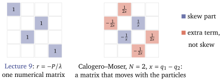
Read (B.20) against Lecture 9’s $\rmat=-\perm/\lambda$ (Figure B.4). The first sum is skew, $\perm(\cdot)\perm=-(\cdot)$ , and looks like the rational $\perm/\lambda$ of §14.10 with its diagonal removed and the spectral parameter replaced by a position difference. The second sum is the extra term: it is not skew, which is why the two terms of (B.19) do not combine into one commutator. (For $N=2$ a different, single-commutator representative exists pointwise; for $N=3$ none does, Proposition B.3.) And $g$ has disappeared: the same $\rmat$ serves every coupling.

Figure B.4. Two

\rmat

-matrices on

\C^{2}\otimes\C^{2}

, rows and columns in the order

11,12,21,22

, each up to its scalar factor. Left, Lecture 9’s rational one: numbers. Right, the Calogero–Moser

\rmat

of (B.20) for two particles: entries that depend on the separation, and an extra term (red) that breaks the skew symmetry, which is why this

\rmat

enters through the two-term form (B.19).

Theorem B.20 (Involution). If $L$ satisfies (B.19) for any matrix-valued functions $\leg{\rmat}{12}$ , $\leg{\rmat}{21}$ on phase space, then $\pb{\tr L^{n}}{\tr L^{m}}=0$ for all $n,m$ . In particular the Calogero–Moser integrals $F_k$ are in involution.

Proof. Step 1 of Theorem 9.14, the chain rule (9.14), never looked at the bracket. Substituting (B.19), $\pb{\tr L^{n}}{\tr L^{m}} =nm\Big[\tr\big(A\comm{\leg{\rmat}{12}}{\leg{L}{1}}\big) -\tr\big(A\comm{\leg{\rmat}{21}}{\leg{L}{2}}\big)\Big], \qquad A=\leg{L}{1}^{\,n-1}\leg{L}{2}^{\,m-1}.$ $A$ commutes with $\leg{L}{1}$ and with $\leg{L}{2}$ separately (Remark 9.3), and Step 3’s cyclicity argument kills each trace. The values of $\rmat$ at the point where the bracket is evaluated are all that enter; that they vary from point to point costs nothing.

So the machinery did not fail at its first real test. What Lecture 9’s reading proved was more than it assumed: the involution theorem needs only that the bracket is a sum of commutators with $\leg{L}{1}$ and with $\leg{L}{2}$ , and Babelon–Viallet (§9.11) says that some such form always exists behind involution. A constant, skew $\rmat$ is the exception — the open Toda chain has one — and a dynamical $\rmat$ the general situation, as Babelon and Viallet describe it. What does change is Jacobi: Theorem 14.7 (Lecture 14’s reading) was proved for a numerical skew $\rmat$ . For their elliptic dynamical $\rmat$ , Babelon–Bernard–Talon show by direct calculation a generalised Yang–Baxter equation (7.21), with new terms that are Poisson brackets of $L$ with $\rmat$ , and that it implies Jacobi cited; in general Jacobi gives a weaker condition, and $\rmat$ has gauge freedom. Here Jacobi is not in question: the bracket is the canonical one.

B.14 Scattering, and the comparison with Toda

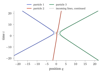
In the rational model the particles repel and the potential dies away, so, as in §12.4, they separate (Moser). Once they have, $L\to\operatorname{diag}(p)$ , and the one-line argument after Theorem 12.2 (Lecture 12) applies word for word: the asymptotic momenta are the eigenvalues $\lambda_1<\dots<\lambda_N$ of $L$ , arriving in decreasing order along the line and leaving in increasing order (Figure B.5). The scattering is elastic and non-diffractive.

Figure B.5. Three particles of the rational gas,

g=1

: momenta (solid) and the eigenvalues of Moser’s

L

(dashed). The momenta are exchanged; the eigenvalues do not move (scripts/figures/cm_scattering.py, which asserts the spectrum and the energy constant to

10^{-9}

and both asymptotic orders).

The positions are where Calogero–Moser and Toda part company.

Proposition B.21 (Two particles). For $N=2$ , with the gap $s=q_2-q_1>0$ and relative speed $v=\lambda_2-\lambda_1$ , every solution has $s(t)^{2}=v^{2}(t-t_0)^{2}+\frac{4g^{2}}{v^{2}}, \qquad\text{so}\qquad s(t)=v\abs{t-t_0}+O(1/t).$ (B.21) The incoming straight lines continue into the outgoing ones with no displacement.

Proof. The gap obeys $\ddot s=4g^{2}/s^{3}$ and conserves $E=\tfrac14\dot s^{2}+g^{2}/s^{2}=\tfrac14v^{2}$ . Then $\frac{\dd^{2}}{\dd t^{2}}s^{2}=2\dot s^{2}+2s\ddot s =2\dot s^{2}+8g^{2}/s^{2}=2v^{2}$ , so $s^{2}$ is a quadratic in $t$ with leading coefficient $v^{2}$ and minimum at the turning point $t_0$ , where $\dot s=0$ and $s^{2}=4g^{2}/v^{2}$ ; and $s>0$ picks the positive root. With the centre of mass $q_c=\tfrac12(q_1+q_2)=q_c(0)+\bar pt$ moving at the mean momentum $\bar p$ , $q_{1,2}=q_c\mp\tfrac12s$ approach $q_c(0)+\bar pt\mp\tfrac12v\abs{t-t_0}$ , the same two straight lines before and after.

Compare Proposition 12.1: the Toda lines are displaced by $\mp2\ln v$ ; here by nothing. For $N$ particles the same holds (Figure B.6).

Theorem B.22 (Moser cited). In the rational model, each line carrying $\lambda_k$ leaves on the continuation of the line on which it arrived: the momenta are permuted, and every position shift is zero. (Moser 1975; Perelomov, §3.3, eqs. 3.3.15–3.3.16.)

The reason is Theorem B.9: the positions $q_j(t)$ are the eigenvalues of the matrix $Q(0)+t\,L(0)$ , with $Q=\operatorname{diag}(q)$ (Perelomov, (3.3.11)). For large $\abs t$ that is $t\big(L(0)+Q(0)/t\big)$ , whose eigenvalues are $t\lambda_k+\beta_k+O(1/t)$ , with $\beta_k$ the diagonal entry of $Q(0)$ in the $k$ -th eigenvector of $L(0)$ , by first-order perturbation theory. The same $\beta_k$ for $t\to+\infty$ and $t\to-\infty$ : the line carrying $\lambda_k$ has one offset, before and after.

Figure B.6. World lines of three particles (time upward), with each incoming straight line continued through the collision (dotted). Every outgoing world line lies on one of them: the momenta are permuted and nothing is displaced, unlike Figure 12.3. (cm_scattering.py asserts every displacement below

2\times10^{-2}

, the

1/t

tail at

\abs t=2000

.)

The non-compact fibre again. The hypothesis audit of §9.12 (Lecture 9’s reading) runs as it did for Toda. Involution and independence hold; the flow of $F_1$ translates the whole gas, so no level set is compact; and the flows are complete, by the argument of Proposition 9.23 with one addition: on a level set $\abs{L_{jk}}=g/\abs{q_{jk}}$ is bounded, so the particles stay a fixed distance apart and the chamber’s walls are never reached (for the Hamiltonian flow itself, Theorem B.9(a) says so directly). The torus conclusion fails, and what replaces it is scattering. (One line of generalisation: Ruijsenaars and Schneider (1986) found a relativistic deformation of these models, still integrable, the elliptic case included (Ruijsenaars 1987); a reading below.)

B.15 The trapped Lax pair

Add a harmonic trap: $H_\freq=H+\tfrac12\freq^{2}\sum_jq_j^{2}$ , rational $V$ . The gas is now confined, and $L$ is no longer isospectral, but $L^{\pm}=L\pm\ii\freq Q,\qquad \dot L^{\pm}=\comm{M}{L^{\pm}}\pm\ii\freq L^{\pm},$ (B.22) with the same $M$ (Perelomov, §3.1; checked symbolically for $N=3$ ). The extra terms cancel in the product: $\frac{\dd}{\dd t}(L^{+}L^{-}) =\comm{M}{L^{+}L^{-}}$ , so the $\tr(L^{+}L^{-})^{k}$ are first integrals. That $N$ of them are independent and in involution — so that the trapped gas is Liouville integrable — is a further computation (Perelomov, §3.1; Avan–Talon, §4) cited; a Lax equation alone does not give it (Lecture 8’s IOU, §8.3). More is true: the positions are the eigenvalues of $Q(0)\cos\freq t+\freq^{-1}L(0)\sin\freq t$ (Perelomov, (3.3.25) cited), so every orbit is periodic with period $2\pi/\freq$ , whatever its energy — Corollary B.10 proves it by reduction. scripts/check-l11-algebra.py checks the return at $t=2\pi/\freq$ numerically. This confined model, isochronous and (cited) integrable, is the one §B.6 quantises.

B.16 The projection theorem, proved

Proof of Theorem B.9. Run the argument backwards: start from the free motion (B.6), defined for all $t$ , with $P(t)=L(0)$ and $\comm{X(t)}{P}=\comm{Q(0)}{L(0)}=\xi$ (Corollary B.5). By Lemma B.7 the eigenvalues $\tilde q_1(t)<\dots<\tilde q_N(t)$ of $X(t)$ stay distinct, so the orthogonal projections $\Pi_j(t)$ onto the eigenlines are smooth in $t$ (for a simple eigenvalue, $\Pi_j=\frac1{2\pi\ii}\oint(z-X)^{-1}\dd z$ around $\tilde q_j$ alone). Let $U(t)$ have columns $u_j=\Pi_je$ . In the notation of the lemma, $u_j=v_jw_j$ with $v_j$ a unit eigenvector and $\abs{w_j}=1$ , so $U$ is unitary, and $u_j^{\dagger}e=\abs{w_j}^{2}=1$ , so $U^{\dagger}e=e$ : the gauge of Theorem B.8(a), chosen smoothly, with $U(0)=\Id$ since $X(0)$ is diagonal. So $U(t)\in\U(N)_\xi$ , $U^{\dagger}XU=\tilde Q(t)$ , and $\tilde L(t):=U^{\dagger}L(0)U$ has the form (B.5) with some diagonal $\tilde p(t)$ . Put $A=U^{\dagger}\dot U$ , anti-Hermitian.

Differentiate $\tilde Q=U^{\dagger}XU$ , using $\dot X=L(0)$ , $\dot U^{\dagger}=-AU^{\dagger}$ and $XU=U\tilde Q$ : $\dot{\tilde Q}=\tilde L+\comm{\tilde Q}{A}$ . $\comm{\tilde Q}{A}$ has zero diagonal, so $\dot{\tilde q}_j=\tilde p_j$ ; off the diagonal the left side is $0$ , so $A_{jk}=-\tilde L_{jk}/(\tilde q_j-\tilde q_k)=-\ii g/(\tilde q_j-\tilde q_k)^{2}$ . The diagonal of $A$ is the gauge condition: $U^{\dagger}e=e$ for all $t$ , so $0=\dot U^{\dagger}e=-Ae$ , every row of $A$ sums to zero, and $A_{jj}=-\sum_{l\ne j}A_{jl}$ . So $M=-A$ is (B.7). Differentiate $\tilde L=U^{\dagger}L(0)U$ : $\dot{\tilde L}=\comm{M}{\tilde L}$ , whose diagonal is $\sum_{l\ne j}\big(M_{jl}\tilde L_{lj}-\tilde L_{jl}M_{lj}\big) =2g^{2}\sum_{l\ne j}(\tilde q_j-\tilde q_l)^{-3}=-\partial H/\partial q_j$ . So $(\tilde q,\tilde p)$ solves Hamilton’s equations for all $t$ from $(q(0),p(0))$ , and by uniqueness of solutions (Theorem 1.5) it is $(q,p)$ . That proves (a) and (b).

B.17 Conjugation, its momentum map, and the reduction theorem

The core used a handful of facts about conjugation without proof. Here they are, with the general theorem behind the reduction.

Lecture 5’s proof (§5.5) used an action of $\R^{n}$ , its orbits and its stabilisers (Definition 5.8). The same words, for any group:

Definition B.23 (Group action, orbit, stabiliser). An action of a group $G$ on a set $\mathcal S$ assigns to each $U\in G$ a map $\Phi_U:\mathcal S\to\mathcal S$ with $\Phi_{\Id}=\id$ and $\Phi_U\circ\Phi_V=\Phi_{UV}$ . The orbit of $s\in\mathcal S$ is $\{\Phi_U(s):U\in G\}$ ; its stabiliser is $G_s=\{U:\Phi_U(s)=s\}$ , a subgroup.

Orbits partition $\mathcal S$ . Points on one orbit have conjugate stabilisers, $G_{\Phi_V(s)}=VG_sV^{-1}$ ; for the abelian group of Lemma 5.9 that made them equal.

The example. $\Herm(N)$ , the $N\times N$ Hermitian matrices, is a real vector space of dimension $N^{2}$ ( $N$ real diagonal entries, $N(N-1)/2$ complex ones above the diagonal), and $\inner{A}{B}=\tr(AB)$ (B.23) is a Euclidean inner product on it: $\tr(A^{2})=\sum_{j,k}\abs{A_{jk}}^{2}$ . The unitary group $\U(N)$ acts by conjugation, $\Phi_U(X)=UXU^{\dagger}$ , and preserves (B.23): $\tr(UAU^{\dagger}UBU^{\dagger})=\tr(AB)$ . So conjugation is a group of rotations of the Euclidean space $\Herm(N)\cong\R^{N^{2}}$ . Scalars $U=e^{\ii\theta}\Id$ act trivially; this will matter every time we count.

Proposition B.24 (Orbits of conjugation).

(a)
The orbit of $X$ is the set of Hermitian matrices with the same eigenvalues, counted with multiplicity. Each orbit contains exactly one diagonal matrix $Q=\operatorname{diag}(q_1,\dots,q_N)$ with $q_1\le\dots\le q_N$ .
(b)
Write $\ulie(N)$ for the anti-Hermitian matrices, the velocities $\dot U(0)$ of curves in $\U(N)$ through $\Id$ . The velocities of curves in the orbit through $X$ are the matrices $\comm{A}{X}$ , $A\in\ulie(N)$ .
(c)
If $X=Q$ is regular — all $q_j$ distinct — then $\comm{A}{Q}=0$ exactly for diagonal $A$ , the stabiliser $\U(N)_Q$ is the group $T^{N}$ of diagonal unitaries, and the orbit has dimension $N^{2}-N$ .

Proof. (a) is the spectral theorem: $X=UQU^{\dagger}$ with $U$ unitary and $Q$ real diagonal, and the order of the $q_j$ can be chosen by permuting the columns of $U$ . (b) If $U(s)$ is a curve in $\U(N)$ with $U(0)=\Id$ and $\dot U(0)=A$ , then $U^{\dagger}U=\Id$ gives $A^{\dagger}+A=0$ , and $\frac{\dd}{\dd s}U(s)XU(s)^{\dagger}\big|_{0}=AX+XA^{\dagger}=\comm{A}{X}$ ; conversely $U(s)=e^{sA}$ realises any $A$ . (c) Entry by entry, $\comm{A}{Q}_{jk}=(q_k-q_j)A_{jk}$ , which vanishes for all $j\ne k$ exactly when $A$ is diagonal. A unitary $U$ with $UQ=QU$ maps each eigenline of $Q$ to itself, so is diagonal. The velocities $\comm{A}{Q}$ fill the $N^{2}-N$ real dimensions of the off-diagonal part, so that is the orbit’s dimension (its tangent space at $Q$ ).

The phase space, and the momentum map. Throughout, $N\ge2$ . The phase space of a free particle in $\Herm(N)$ is $\phase=\Herm(N)\times\Herm(N)$ , points $(X,P)$ : a position matrix and a momentum matrix. ( $P$ here is a matrix of momenta; the permutation operator of Proposition B.3, which the course also writes $P$ , does not appear in the reduction. And $X$ is a matrix, not a vector field: Hamiltonian vector fields keep their subscript, $\hvf{f}$ .) Choose an orthonormal basis $T_1,\dots,T_{N^{2}}$ of $\Herm(N)$ for (B.23) — for instance $E_{jj}$ , $(E_{jk}+E_{kj})/\sqrt2$ and $\ii(E_{jk}-E_{kj})/\sqrt2$ for $j<k$ — and write $X=\sum_ax_aT_a$ , $P=\sum_ap_aT_a$ . We declare $(x_a,p_a)$ canonical: $\symp=\sum_{a=1}^{N^{2}}\dd x_a\wedge\dd p_a=:\tr(\dd X\wedge\dd P), \qquad H=\tfrac12\tr P^{2}=\tfrac12\sum_ap_a^{2}.$ (B.24) So $\phase$ is just $\R^{2N^{2}}$ with Lecture 2’s bracket, and $H$ is a free particle: $\dot X=P$ , $\dot P=0$ , which is (B.3). For a function $f(X,P)$ write $\partial f/\partial X=\sum_a(\partial f/\partial x_a)T_a$ , a Hermitian matrix; then $\pb fh=\tr\big(\frac{\partial f}{\partial X}\frac{\partial h}{\partial P} -\frac{\partial f}{\partial P}\frac{\partial h}{\partial X}\big)$ , and a linear function has the obvious gradient: $\partial\tr(BX)/\partial X=B$ for Hermitian $B$ .

$\U(N)$ acts on $\phase$ by conjugating both matrices, $\Phi_U(X,P)=(UXU^{\dagger},UPU^{\dagger})$ . In the coordinates $(x_a,p_a)$ this is the same rotation $O$ of $\R^{N^{2}}$ applied to $x$ and to $p$ , and any such map is a symplectomorphism (Definition 4.6): $\sum\dd x_a\wedge\dd p_a$ is the bilinear form $x\cdot p'-p\cdot x'$ on pairs of tangent vectors, which $O$ preserves. And $H$ is invariant: $\tr(UPU^{\dagger})^{2}=\tr P^{2}$ .

A one-parameter subgroup $U(s)=e^{sA}$ , $A\in\ulie(N)$ , moves points of $\phase$ with velocity $(\comm{A}{X},\comm{A}{P})$ at $s=0$ (Proposition B.24(b)). Lecture 2’s Noether principle says a function whose flow is a symmetry of $H$ is conserved; a momentum map is the bookkeeping device that produces such a function for every $A$ at once.

Definition B.25 (Momentum map). A momentum map for the action of $\U(N)$ on $\phase$ is a function $\momap$ from $\phase$ to $\ulie(N)$ such that, for every $A\in\ulie(N)$ , the real function $\momap_A=\tr(A\momap)$ has Hamiltonian vector field equal to the velocity field of $e^{sA}$ : $\hvf{\momap_A}X=\comm{A}{X},\qquad \hvf{\momap_A}P=\comm{A}{P},$ the vector field acting on the matrix coordinates entry by entry.

The literature writes $\mu$ , which here is the spectral parameter. The trace pairing replaces the usual map into the dual of the Lie algebra: $\tr(AB)$ is real and non-degenerate on $\ulie(N)$ , so one matrix $\momap(X,P)$ records all the $\momap_A$ . For translations of a particle in $\R^{3}$ the momentum map is the momentum; for rotations it is the angular momentum (Example 4.3).

Proposition B.26 (The momentum map is a commutator). $\momap(X,P)=\comm{X}{P}$ is a momentum map for conjugation.

Proof. $\comm{X}{P}^{\dagger}=\comm{P}{X}=-\comm{X}{P}$ , so $\momap$ is anti-Hermitian, and $\momap_A=\tr(A\comm{X}{P})$ is real, since the trace of a product of two anti-Hermitian matrices is. By cyclicity $\momap_A=\tr(P\comm{A}{X})=\tr(X\comm{P}{A})$ , and $\comm{A}{X}$ , $\comm{P}{A}$ are Hermitian, so the linear-gradient rule gives $\partial\momap_A/\partial P=\comm{A}{X}$ and $\partial\momap_A/\partial X=\comm{P}{A}$ . With $\hvf{f}h=\pb hf$ : $\hvf{\momap_A}X=\pb{X}{\momap_A}=\frac{\partial\momap_A}{\partial P}=\comm{A}{X}, \qquad \hvf{\momap_A}P=\pb{P}{\momap_A}=-\frac{\partial\momap_A}{\partial X}=\comm{A}{P}.$

For any $\U(N)$ -invariant $H$ , not only the two of Corollary B.5, $\momap$ is conserved: $\pb{\momap_A}{H}=-\hvf{\momap_A}H=-\frac{\dd}{\dd s}H(\Phi_{e^{sA}})\big|_0=0$ , Noether as in Lecture 2.

Write $\momap^{-1}(\xi)=\{(X,P):\comm{X}{P}=\xi\}$ for the level set. The general theorem behind the reduction is this; in the core it supplies only the reduced symplectic form and its brackets, and everything else is proved on the example.

Theorem B.27 (Marsden–Weinstein reduction cited). Let a compact group $G$ act on $(\phase,\symp)$ by symplectomorphisms with an equivariant momentum map $\momap$ , and let $\xi$ be a value of $\momap$ at which $\dd\momap$ is onto at every point of $\momap^{-1}(\xi)$ (a regular value), and on which the stabiliser $G_\xi$ of $\xi$ acts freely (a subgroup acting trivially on all of $\phase$ , like the scalars here, is divided out of $G$ first). Then $\phase_\xi=\momap^{-1}(\xi)/G_\xi$ is a manifold of dimension $\dim\phase-\dim G-\dim G_\xi$ , carrying a unique symplectic form $\symp_\xi$ whose pull-back to $\momap^{-1}(\xi)$ is the restriction of $\symp$ . A $G$ -invariant Hamiltonian defines a function on $\phase_\xi$ , whose flow is the image of the original flow, and Poisson brackets of $G$ -invariant functions pass to $\phase_\xi$ . (Marsden and Weinstein 1974; da Silva, Thm 23.1 and §24.4.)

$\momap=\comm{X}{P}$ is anti-Hermitian and traceless ( $\tr\comm{X}{P}=0$ ), so a level $\xi$ must be too. This matches the scalars acting trivially: the group that acts effectively is $\mathrm{PU}(N)=\U(N)/\U(1)$ , and through the trace pairing its Lie algebra is $\su(N)$ , the traceless anti-Hermitian matrices. From here on $\momap$ is regarded as a map $\phase\to\su(N)$ , of dimension $N^{2}-1$ , and that is the $\momap$ to which Theorem B.27 is applied, with $G=\mathrm{PU}(N)$ . Fix a level $\xi$ . By Corollary B.5(b), $\Phi_U$ carries $\momap^{-1}(\xi)$ onto $\momap^{-1}(U\xi U^{\dagger})$ . For $\xi\ne0$ that is generally a different level set: $\U(N)$ does not act on $\momap^{-1}(\xi)$ , so $\momap^{-1}(\xi)/\U(N)$ does not make sense. What does act is the stabiliser $\U(N)_\xi=\{U\in\U(N):U\xi U^{\dagger}=\xi\},$ and $\momap^{-1}(\xi)/\U(N)_\xi$ is what replaces it. Physicists call $\U(N)_\xi$ the residual gauge group: two points of $\momap^{-1}(\xi)$ related by one of its elements are the same physical state.

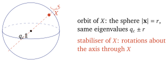
The orbit of $\xi$ sketched is $\{\ii g(ww^{\dagger}-\Id):w\in\C^{N},\ \abs{w}^{2}=N\}$ , of dimension $2N-2$ : $U\xi U^{\dagger}=\ii g(ww^{\dagger}-\Id)$ with $w=Ue$ , and $\U(N)$ moves $e$ to every vector of the same length. The dimension is $\dim\U(N)-\dim\U(N)_\xi=N^{2}-\big(1+(N-1)^{2}\big)=2N-2$ : as in Proposition B.24(b), the orbit’s velocities are the $\comm{A}{\xi}$ , and the $A$ with $\comm{A}{\xi}=0$ are the stabiliser’s.

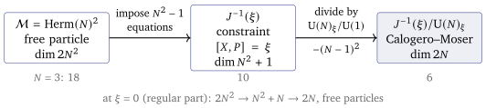
Dimensions. The constraint $\comm{X}{P}=\xi$ is $N^{2}-1$ real equations (the trace is automatic), independent on $\momap^{-1}(\xi)$ : $\xi$ is a regular value of $\momap:\phase\to\su(N)$ , and $\momap^{-1}(\xi)$ is a manifold of dimension $N^{2}+1$ . At $\xi=0$ the torus $T^{N}$ fixes a point $(Q,\operatorname{diag}(p))$ , $N-1$ equations become dependent there, and the level set has dimension $N^{2}+N$ ; at $(X,P)=(0,0)$ it is not a manifold at all. $0$ is not a regular value, and Theorem B.27 does not apply to it as stated. (Proofs in the next reading.)

Proof of Theorem B.8(c). On the slice $\dd X=\operatorname{diag}(\dd q_j)$ has no off-diagonal part, so in $\tr(\dd X\wedge\dd P)=\sum_{j,k}\dd X_{jk}\wedge\dd P_{kj}$ only the terms $j=k$ survive: $\sum_j\dd q_j\wedge\dd L_{jj}=\sum_j\dd q_j\wedge\dd p_j$ . By Theorem B.27 the reduced form is the one whose pull-back to the level set is the restriction of $\symp$ ; the slice meets each gauge orbit once, so this is it.

The reduction at zero, and the counting.

Proposition B.28 (Reduction at zero gives free particles). Every point of $\momap^{-1}(0)$ with $X$ regular is $\U(N)$ -equivalent to $(Q,\operatorname{diag}(p))$ with $q_1<\dots<q_N$ , and to exactly one such. On these points $H=\tfrac12\sum_jp_j^{2}$ : free particles.

Proof. Conjugate $X$ to $Q$ (Proposition B.24(a)); the constraint becomes $\comm{Q}{P}_{jk}=(q_j-q_k)P_{jk}=0$ , and $q_j\ne q_k$ forces $P_{jk}=0$ for $j\ne k$ . Uniqueness: a unitary carrying one such pair to another fixes the ordered $Q$ , so is diagonal (Proposition B.24(c)), and diagonal unitaries fix every diagonal $P$ .

The dimension is right, $2N$ ; the Hamiltonian is wrong. In Figure B.1 this is a diagonal $P_0$ , whose eigenvalues $q_j+tp_j$ cross; in Example B.4, zero angular momentum, a line through the origin and no barrier. At $\xi$ of (B.4): $N^{2}-1$ constraint equations, and a residual gauge group of dimension $1+(N-1)^{2}$ whose scalars act trivially, leave $2N^{2}-(N^{2}-1)-(N-1)^{2}=2N$ , as the slice says (Figure B.7).

Figure B.7. The reduction diagram: a free particle; the surface where the conserved

\comm{X}{P}

takes one value; the quotient by what preserves that value. Only the non-zero level gives an interaction.

Figure B.8. What survives of

P

once

X=Q

is diagonal. The constraint fixes every off-diagonal entry: at level zero to

0

(free particles), at the level (B.4) to

\ii g/(q_j-q_k)

(Calogero–Moser).

Figure B.9. Free motion in matrix space,

N=2

(Example B.4). Left: the traceless part

\mathbf x

of

X(t)

moves on a straight line in

\R^{3}

; the closest it gets to the origin is the impact parameter

\abs{\boldsymbol\ell}/\abs{\mathbf v}

. Right: the two eigenvalues are

\pm\abs{\mathbf x(t)}

, so they approach, turn and separate — the centrifugal barrier, seen as a repulsion.

Figure B.10. Gauge fixing. The level set is a union of orbits of the residual gauge group (grey); the slice (indigo) meets each exactly once, and is the reduced phase space.

B.18 Regular and singular levels

Why $\xi$ is a regular value of $\momap$ and $0$ is not. For a tangent vector $v$ at a point of $\phase$ , $\tr(A\,\dd\momap(v))=\dd\momap_A(v) =\symp(\hvf{\momap_A},v)$ , which vanishes for every $v$ exactly when $\hvf{\momap_A}=0$ there, i.e. when $e^{sA}$ fixes the point. So the image of $\dd\momap$ is everything orthogonal to the Lie algebra of the point’s stabiliser. On $\momap^{-1}(\xi)$ , by Theorem B.8(a), every point is conjugate to a slice point $(Q,L)$ ; a unitary fixing $Q$ is diagonal, and $DLD^{\dagger}=L$ with every $L_{jk}\ne0$ forces $D_{jj}=D_{kk}$ . Only the scalars fix the point, so $\dd\momap$ is onto the traceless anti-Hermitian matrices, of dimension $N^{2}-1$ . At $(Q,\operatorname{diag}(p))\in \momap^{-1}(0)$ with $Q$ regular the stabiliser is $T^{N}$ , and the rank drops to $N^{2}-N$ . Near such a point $\momap^{-1}(0)$ consists of pairs diagonalised together, $X$ still with distinct eigenvalues: $N$ eigenvalues of $X$ , $N$ of $P$ and an orbit $\U(N)/T^{N}$ of dimension $N^{2}-N$ , in all $N^{2}+N$ , not $N^{2}+1$ . (The same holds wherever the joint eigenspaces of $X$ and $P$ are lines, e.g. at $X=0$ with $P$ regular; $X$ regular is merely the part Proposition B.28 uses.) At $(X,P)=(0,0)$ the level set is not a manifold: it is a cone (invariant under $(X,P)\mapsto(sX,sP)$ ), and a cone that is a manifold at its vertex is a linear subspace; this one is not, since $(\sigma_3,0)$ and $(0,\sigma_1)$ lie on it and their sum does not.

B.19 Root systems and the other Calogero–Moser models

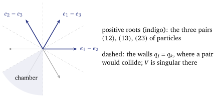
The differences $q_j-q_k$ are not an accident of notation. (Olshanetsky and Perelomov’s generalisation, below, keeps every model of Figure B.2 integrable; this is where $\sllie_N$ comes from.) The diagonal matrices $Q$ act on the matrix units by $\comm{Q}{E_{jk}}=(q_j-q_k)E_{jk}$ : the numbers $q_j-q_k$ are the eigenvalues of $\ad_Q$ , which in Lie theory are the values at $Q$ of the roots $e_j-e_k$ of $\sllie_N$ (the root system $A_{N-1}$ ). The constraint of Theorem B.8 is one equation per root space, and the Calogero–Moser potential is a sum over the positive roots $\alpha$ of $g^{2}/\alpha(q)^{2}$ . For $N=3$ , in the plane $q_1+q_2+q_3=0$ where the centre of mass has been removed, the three positive roots are drawn in Figure B.11: each is a pair of particles, and its hyperplane $\alpha(q)=0$ is where that pair would collide. The chamber $q_1<q_2<q_3$ of Theorem B.8 is a Weyl chamber, cut out by those walls.

Olshanetsky and Perelomov (1976) replaced $A_{N-1}$ by other root systems $R$ : $H=\tfrac12\abs{p}^{2}+\sum_{\alpha\in R_+}g_\alpha^{2}\,V\big(\alpha(q)\big),$ with couplings $g_\alpha$ equal on roots related by the Weyl group. For $BC_N$ (which contains $B_N$ , $C_N$ , $D_N$ as special couplings) and $V$ rational, hyperbolic or trigonometric, they constructed a Lax pair, and so proved Liouville integrability, for couplings obeying one further relation: with $g$ on the roots $e_j\pm e_k$ , $g_1$ on $e_j$ and $g_2$ on $2e_j$ , either $g_1=0$ or $g_1^{2}+\sqrt2\,g_1g_2-2g^{2}=0$ (Perelomov, §3.9, Proposition 2) cited. The exceptional systems are integrable too, but Perelomov records no Lax pair for them. For $B_N$ , $C_N$ , $D_N$ the positive roots include $e_j+e_k$ as well as $e_j-e_k$ (and $e_j$ or $2e_j$ ), so particle $j$ interacts also with the mirror image of particle $k$ and, for $B_N$ and $C_N$ , with a wall at the origin. For those couplings they obtained the rational and hyperbolic models by projecting free motion on symmetric spaces of zero and negative curvature, and the trigonometric one from positive curvature — the construction of this lecture, with $\Herm(N)$ one example (Perelomov, §3.3). In the same spirit, Kazhdan, Kostant and Sternberg obtained the trigonometric model $1/\sin^{2}$ by replacing the matrix $X$ with a unitary matrix, so that its eigenvalues live on a circle cited. Root systems return in optional lecture C, as the Dynkin diagrams indexing nested Bethe equations.

Figure B.11. The root system

A_2

of

\sllie_3

, drawn in the plane

q_1+q_2+q_3=0

. Each positive root is one interacting pair; the six walls bound the Weyl chambers, and the particles stay in one of them. (The chamber is shaded only schematically; its sides are two of the walls.)

B.20 Ruijsenaars–Schneider

Ruijsenaars and Schneider (1986) found a one-parameter deformation of every Calogero–Moser model, still integrable, that behaves like a relativistic particle system: with $c$ a “speed of light” and unit masses, the rational one is $H_{\mathrm{RS}}=c^{2}\sum_{j=1}^{N}\cosh\frac{p_j}{c} \prod_{k\ne j}\Big(1+\frac{g^{2}}{c^{2}(q_j-q_k)^{2}}\Big)^{1/2} =Nc^{2}+H_{\mathrm{CM}}+O(c^{-2})$ (Arutyunov, (1.67); the expansion is checked in scripts/check-l12-algebra.py). It too comes from reduction: the rational model from the cotangent bundle of the group $\GL(N)$ in place of the matrix space (Arutyunov, §2.2.1), and the hyperbolic one from a Poisson–Lie deformation of that, the “Heisenberg double” (§2.2.2) cited. This course does not develop either. The elliptic case is Ruijsenaars (1987). Its quantum version is beyond this course.

B.21 The quantum models, carefully: units, the circle, the domain

Remark B.29 (Units, and a named clash). This lecture uses $\hbar=m=1$ , kinetic operator $-\tfrac12\sum_j\partial_j^{2}$ , so that (B.1)’s $H=\tfrac12\sum p^{2}+g^{2}\sum V$ is its literal classical limit — and not the $\hbar=2m=1$ of Lecture 11, Lecture 16 and Lecture 17, which belongs to Lieb–Liniger. Mixing the two in one formula is how a model with no Jastrow ground state gets printed. The trap frequency is $\freq$ , as in (B.22); $\omega$ is the symplectic form and nothing else.

The circle. The trigonometric model, Sutherland’s, is $H_{\mathrm S}=-\frac12\sum_{j=1}^{N}\partial_j^{2} +\sum_{i<j}\frac{\beta(\beta-1)}{\sin^{2}(x_i-x_j)}$ (B.25) on a circle of circumference $\pi$ , and its Jastrow state is $\psi_0^{\mathrm S}=\prod_{i<j}\bigl(\sin(x_j-x_i)\bigr)^{\beta},\qquad H_{\mathrm S}\psi_0^{\mathrm S}=E_0^{\mathrm S}\psi_0^{\mathrm S},\qquad E_0^{\mathrm S}=\frac{\beta^{2}N(N^{2}-1)}6 ,$ (B.26) by the computation of Theorem B.11 with one change. For $\psi_0^{\mathrm S}$ replace $x_{ij}^{-1}$ by $\cot x_{ij}$ . Now $\partial_i^{2}W=-\beta\sum_{j\ne i}\csc^{2}x_{ij}$ and $\cot^{2}=\csc^{2}-1$ , so the two-index terms again cancel the potential and leave $\beta^{2}N(N-1)/2$ ; and the three-index sum is no longer zero but is fixed by the cotangent identity $\cot a\cot b+\cot b\cot c+\cot c\cot a=1$ whenever $a+b+c=0$ , applied to $a=x_{ij}$ , $b=x_{jk}$ , $c=x_{ki}$ . Each unordered triple contributes $-2$ , so that sum is $-N(N-1)(N-2)/3$ , and $-\tfrac12\beta^{2}$ times it is $+\beta^{2}N(N-1)(N-2)/6$ . Hence $E_0^{\mathrm S}=\beta^{2}N(N-1)/2+\beta^{2}N(N-1)(N-2)/6$ , which is (B.26) checked: symbolically at $N=3$ , in both the trigonometric and the $z$ variables, and by exact evaluation at $N=4,5,6$ .

The coupling. With $\hbar$ restored the coupling is $\hbar^{2}\beta(\beta-1)$ , so $\beta=\tfrac12+\sqrt{\tfrac14+g^{2}/\hbar^{2}}$ and $\hbar\beta\to g$ as $\hbar\to0$ : the classical $g$ is the limit of $\hbar\beta$ , and the classical regime is $\beta\to\infty$ checked.

The domain. Near a collision the relative coordinate $r=x_i-x_j$ sees $-\partial_r^{2}+\beta(\beta-1)/r^{2}$ , whose solutions behave as $r^{p}$ with $p(p-1)=\beta(\beta-1)$ : two exponents, $p=\beta\quad\text{and}\quad p=1-\beta ,$ (B.27) which the coupling does not distinguish checked. Fix $\beta\ge\tfrac12$ , choosing the larger — a labelling convention, not a stability condition, since $\beta(\beta-1)=(\beta-\tfrac12)^{2}-\tfrac14$ never falls below the Hardy bound $-\tfrac14$ , which it attains at $\beta=\tfrac12$ , where the exponents coincide and the second solution is $r^{1/2}\ln r$ .

Definition B.30 (The model, completely). Take the ordered chamber — $x_1<\dots<x_N$ on the line, and $0\le x_1<\dots<x_N<\pi$ on the circle, where $x_N-x_1\to\pi$ counts as a collision too — and define the operator as the Friedrichs extension of (B.8) or (B.25) from the smooth functions compactly supported away from every collision. On this domain an eigenfunction behaves at a collision as $\psi=O\bigl(\abs{x_i-x_j}^{\beta}\bigr),\qquad x_i\to x_j ,$ (B.28) the larger of the two exponents in (B.27). For $\beta\ge\tfrac32$ the Friedrichs extension is the only self-adjoint one, the other branch $r^{1-\beta}$ being not even locally square-integrable; for $\tfrac12\le\beta<\tfrac32$ the operator is not essentially self-adjoint, and (B.28) is what picks this extension out of the family cited: Reed and Simon II, §X.1 and its appendix. For (B.25) there is a second, global condition: the model is bosonic and periodic, so a state extends from the chamber to a symmetric function of period $\pi$ in each coordinate.

Two conventions follow and are used throughout. Restricting to the chamber and extending bosonically to $\R^{N}$ are unitarily equivalent up to $\sqrt{N!}$ , so a symmetric function on $\R^{N}$ and a function on the chamber are the same object; and $\Delta=\prod_{i<j}(x_j-x_i)$ is positive there, so the symmetric function $\Delta^{\beta}$ names is $\abs\Delta^{\beta}$ . And (B.28) describes eigenfunctions, not the whole operator domain, which contains functions with no pure power behaviour at all.

Figure B.12. The single-particle density of the trapped Jastrow state (B.9) at

N=3

, for

\beta=1,2,4

(quadrature,

\freq=1

). The

\beta=1

curve lies on the free-fermion density

\sum_{n<3}\abs{\phi_n}^{2}

, in grey behind it, because

\Delta\,e^{-\freq r^{2}/2}

is their Slater determinant. Raising

\beta

widens the cloud; the generator asserts all three statements.

Why it is the ground state, and why positivity is not the reason

The usual argument is that a positive eigenfunction of a Schrödinger operator on a connected domain is the ground state. That is true, and here it needs a hypothesis that is easy to drop.

Remark B.31 (The partner exponent). Replacing $\beta$ by $1-\beta$ in $\psi_0^{\mathrm S}$ changes neither (B.25) nor the positivity of the function on the chamber, and Theorem B.11’s computation — which used only the exponent — makes it solve the same differential equation with the value $(1-\beta)^{2}N(N^{2}-1)/6$ , strictly smaller than $E_0^{\mathrm S}$ for $\beta>\tfrac12$ checked. So positivity alone cannot identify the ground state. What excludes the partner is Definition B.30, and the test is sharper than it looks: at $N=2$ the partner leaves $L^{2}$ exactly at $\beta=\tfrac32$ , but for $N\ge3$ the binding collision is the total one, where $\Delta^{1-\beta}$ is homogeneous of degree $(1-\beta)N(N-1)/2$ in $N-1$ relative coordinates and its square is integrable only for $\beta<1+1/N$ . A cluster of $m$ particles gives $\beta<1+1/m$ , and $1+1/m$ decreases in $m$ , so the total collision is the sharpest of the $N-1$ tests. At $N=3$ , $\beta=\tfrac75$ every pair test passes and the triple collision diverges checked. So the honest statement is that (B.9) is positive, lies in the form domain of Definition B.30, and is the ground state of that operator sketched.

B.22 The trapped spectrum, drawn

Figure B.13 draws Theorem B.16 at $N=3$ .

Figure B.13. The trapped spectrum at

N=3

for

\beta=\tfrac12,1,3

, beside free bosons. Only

E_0

moves with

\beta

; above it the ladder has spacing

\freq

and multiplicities

1,1,2,3,4,5,7

, the partitions of

n=0,\dots,6

into at most three parts. The generator builds the matrix of (B.13) in exact arithmetic and checks it is degree-triangular with diagonal

\freq\cdot\text{degree}

.

B.23 The Jastrow computation, and Dunkl’s two theorems

Proof of Theorem B.11. For $\psi=e^{W}$ , $\psi^{-1}(-\tfrac12\sum\partial_j^{2})\psi =-\tfrac12\sum_j\bigl(\partial_j^{2}W+(\partial_jW)^{2}\bigr)$ , so everything reduces to two identities. Take $W=\beta\sum_{i<j}\ln(x_j-x_i)$ and write $x_{ij}=x_i-x_j$ . Then $\partial_iW=\beta\sum_{j\ne i}x_{ij}^{-1}$ and $\partial_i^{2}W=-\beta\sum_{j\ne i}x_{ij}^{-2}$ , so $-\frac12\sum_i\bigl(\partial_i^{2}W+(\partial_iW)^{2}\bigr) =\frac\beta2\sum_{i}\sum_{j\ne i}\frac1{x_{ij}^{2}} -\frac{\beta^{2}}2\sum_{i}\sum_{j\ne i}\frac1{x_{ij}^{2}} -\frac{\beta^{2}}2\sum_{i}\sum_{\substack{j,k\ne i\\ j\ne k}} \frac1{x_{ij}x_{ik}} .$ The last sum vanishes: each unordered triple $\{i,j,k\}$ contributes six terms, two copies of $(x_{ij}x_{ik})^{-1}+(x_{ji}x_{jk})^{-1}+(x_{ki}x_{kj})^{-1}$ , which is zero after clearing denominators. The first two give $-\beta(\beta-1)\sum_{i<j}x_{ij}^{-2}$ , which cancels the potential exactly. That is the last claim.

Now add the Gaussian, $W\mapsto W-\freq\sum x_j^{2}/2$ . The new terms are $-\tfrac12\sum_i(-\freq)=\freq N/2$ , then $-\tfrac12\freq^{2}\sum x_j^{2}$ , which cancels the trap, and the cross term $\freq\beta\sum_i\sum_{j\ne i}\frac{x_i}{x_{ij}} =\freq\beta\sum_{i<j}\frac{x_i-x_j}{x_{ij}} =\freq\beta\frac{N(N-1)}2 .$ Together these are $E_0^{\mathrm C}$ .

Example B.32 ( $N=2$ , entirely). Write $s=s_{12}$ , $x=x_1-x_2$ and $A=\beta(1-s)/x$ , so that $D_1=\partial_1+A$ and $D_2=\partial_2-A$ . Then $\comm{D_1}{D_2}=\comm{\partial_1}{-A}+\comm{A}{\partial_2} =-\comm{\partial_1+\partial_2}{A}$ , and $\partial_1+\partial_2$ commutes with $s$ (exchanging the arguments does not change the total derivative) and with $1/x$ ( $x$ is translation invariant). So $\comm{D_1}{D_2}=0$ : at $N=2$ the commutativity is the translation invariance of $x_1-x_2$ .

Proof of Theorem B.13. Everything follows from one commutator with a coordinate. Writing $\delta$ for the Kronecker symbol, $\comm{D_i}{x_l} =\delta_{il}+\beta\sum_{p<q}(\delta_{ip}-\delta_{iq})(\delta_{lp}-\delta_{lq})\,s_{pq}$ (B.29) checked: for $i=l$ the sum is $\sum_{k\ne i}s_{ik}$ , and for $i\ne l$ only the pair $\{i,l\}$ survives, with coefficient $-1$ . Next, relabelling gives $s_{pq}D_ms_{pq}=D_{s_{pq}(m)}$ , whence $\comm{s_{pq}}{D_j}=-(\delta_{jp}-\delta_{jq})(D_p-D_q)s_{pq}$ and $\comm{\comm{D_i}{x_l}}{D_j} =-\beta\sum_{p<q}(\delta_{ip}-\delta_{iq})(\delta_{lp}-\delta_{lq}) (\delta_{jp}-\delta_{jq})\,(D_p-D_q)\,s_{pq}$ (B.30) checked. The right-hand side is symmetric under $i\leftrightarrow j$ , since $i$ and $j$ enter only through the factors $(\delta_{ip}-\delta_{iq})$ and $(\delta_{jp}-\delta_{jq})$ . By the Jacobi identity, therefore, $\comm{\comm{D_i}{D_j}}{x_l} =\comm{\comm{D_i}{x_l}}{D_j}-\comm{\comm{D_j}{x_l}}{D_i}=0$ for every $l$ . So $C=\comm{D_i}{D_j}$ commutes with multiplication by every coordinate, hence by every polynomial, and $Cf=C(f\cdot1)=f\,C(1)=0$ because $D_i1=0$ cited: Dunkl (1989); this argument is Etingof (2009) §6.1.

Proof of Theorem B.14. Both sides in six lines. For symmetric $f$ we have $(1-s_{ij})f=0$ , so $D_if=\partial_if$ ; but $\partial_if$ is not symmetric, so the second $D_i$ must be applied honestly. Using $s_{ij}\partial_i=\partial_js_{ij}$ and $s_{ij}f=f$ , $D_i^{2}f=D_i(\partial_if) =\partial_i^{2}f+\beta\sum_{j\ne i}\frac{\partial_if-\partial_jf}{x_i-x_j} .$ Summing over $i$ doubles each unordered pair, which gives the right-hand side of (B.12).

For the middle expression, write $u=\Delta^{\beta}f$ . Since $\partial_i\Delta^{\beta}/\Delta^{\beta}=\beta\sum_{j\ne i}(x_i-x_j)^{-1}$ , $\Delta^{-\beta}\Bigl(-\frac12\sum_i\partial_i^{2}\Bigr)u =-\frac12\sum_i\partial_i^{2}f -\beta\sum_i\sum_{j\ne i}\frac{\partial_if}{x_i-x_j} +\Bigl(\Delta^{-\beta}\bigl(-\tfrac12{\textstyle\sum}\partial_i^{2}\bigr) \Delta^{\beta}\Bigr)f ,$ and the last bracket is $-\beta(\beta-1)\sum_{i<j}x_{ij}^{-2}$ by the last line of Theorem B.11, which the potential cancels. The surviving double sum is again $\beta\sum_{i<j}(\partial_if-\partial_jf)/(x_i-x_j)$ . The two expressions agree.

Finally $D_i$ is homogeneous of degree $-1$ — both $\partial_i$ and $(1-s_{ij})/(x_i-x_j)$ lower the degree of a homogeneous polynomial by one — so $\sum D_i^{2}$ lowers it by two, or annihilates it; and a permutation $w$ relabels derivatives, differences and transpositions together, so $wD_iw^{-1}=D_{w(i)}$ and $\sum_iD_i^{2}$ is $S_N$ -invariant, hence preserves $\Lambda^{\mathrm{sym}}$ checked at $N=3$ , $N=4$ .

B.24 Sutherland’s excited states

On the circle the natural variable is not $x$ but $z_j=e^{2\ii x_j},$ (B.31) which has period $\pi$ , as the model does. Since $z_i-z_j=2\ii\,e^{\ii(x_i+x_j)}\sin(x_i-x_j)$ and $\abs{z_j}=1$ , the ground state (B.26) is $\prod_{i<j}\abs{z_i-z_j}^{\beta}$ up to the constant $2^{-\beta N(N-1)/2}$ — a constant, not a phase — and $-\tfrac12\sum\partial_{x_j}^{2}=2\sum_j(z_j\partial_{z_j})^{2}$ checked. One more piece of notation: $\kappa$ dominates $\mu$ (same weight) when $\kappa_1+\dots+\kappa_r\ge\mu_1+\dots+\mu_r$ for every $r$ . It is a partial order: at $N=3$ and weight six, $(4,1,1)$ and $(3,3,0)$ are incomparable.

Theorem B.33 (The Sutherland spectrum). Conjugated by $\psi_0^{\mathrm S}$ and written in $z$ , the operator (B.25) preserves the degree and is triangular in the dominance order on the $m_\kappa(z)$ : its eigenfunctions are $\psi_0^{\mathrm S}J_\kappa$ , one for each partition $\kappa_1\ge\dots\ge\kappa_N\ge0$ , with $J_\kappa=m_\kappa+\text{lower}$ , and $E_\kappa=\frac12\sum_{j=1}^{N}k_j^{2}, \qquad k_j=2\kappa_j+\beta\,(N+1-2j) .$ (B.32) The total momentum is $\sum_jk_j=2\abs\kappa$ .

Proof sketched (★). Writing $W=\ln\psi_0^{\mathrm S}$ in the variables $z$ and $A_j=z_j\partial_{z_j}$ , the conjugated operator is $2\sum_j(A_j+w_j)^{2}$ plus the potential, where $w_j=A_jW$ acts by multiplication and is the rational function $\beta\sum_{k\ne j}z_j/(z_j-z_k)-\beta(N-1)/2$ . Expanding, the terms that would produce poles cancel against the potential — exactly as in Theorem B.11, which is the $\kappa=0$ case — and what is left is degree-preserving. Acting on $m_\kappa$ it returns $E_\kappa m_\kappa$ plus multiples of $m_\mu$ with $\mu$ strictly below $\kappa$ in dominance. The coefficients of those $m_\mu$ are then solved for recursively, dividing only by the differences $E_\kappa-E_\mu$ that Remark B.34 says are non-zero. Verified symbolically for $N=2,3$ and $\abs\kappa\le4$ , in $\beta$ , in check-l21-algebra.py.

Remark B.34 (Why “distinct eigenvalues” is the wrong hypothesis). The recursion needs $E_\kappa\ne E_\mu$ only for $\mu$ strictly below $\kappa$ , and that much is true: $E_\kappa=2\sum_j\kappa_j^{2}+2\beta\sum_j\kappa_j(N+1-2j)+E_0^{\mathrm S}$ increases strictly along dominance for $\beta>0$ , since both sums do. Asking instead for distinct diagonal entries would be asking for something false: the incomparable $(4,1,1)$ and $(3,3,0)$ share $E_\kappa=4\beta^{2}+12\beta+36$ for every $\beta$ checked. The $J_\kappa$ are the monic Jack polynomials — Macdonald’s $P_\kappa^{(1/\beta)}$ , which he characterises by this triangularity together with orthogonality; his $J_\kappa^{(\alpha)}$ is a different normalisation cited: Macdonald §VI.10, (10.13)–(10.14); Stanley (1989), which warns about exactly this degeneracy.

Put $\kappa=0$ and $\sum_j(N+1-2j)^{2}=N(N^{2}-1)/3$ returns $E_0^{\mathrm S}$ : the ground state is the empty partition, and the shift is the whole of its energy. The circle also admits Laurent polynomials, $\kappa_N<0$ ; multiplying by $(z_1\cdots z_N)^{m}$ sends $k_j\mapsto k_j+2m$ , a Galilean boost at a different energy and momentum, and $\kappa_N=0$ picks one representative of each boost orbit.

A warning about the standard reference. Beautiful Models §§5.2.5–5.2.6 prints the shift twice as large as (B.32), in contradiction with its own ground-state energy; the last reading of this lecture says exactly where.

Free fermions with shifted momenta

The $k_j$ of (B.32) are a set of quasi-momenta and $E=\tfrac12\sum k_j^{2}$ is the free-particle energy. The interaction lives entirely in the shift $\beta(N+1-2j)$ , which pushes neighbouring momenta at least $2\beta$ apart whatever the state (Figure B.14).

Figure B.14. The quasi-momenta (B.32) for

N=4

. Top: the ground state at

\beta=1

, where the shift alone spreads the four particles over the odd integers

-3,-1,1,3

— free fermions, as Girardeau’s map (Lecture 18’s reading) says. Middle: raising

\beta

dilates the same pattern, gap

2\beta

. Bottom: an excited state,

\kappa=(2,1,0,0)

at

\beta=1

, which moves two quantum numbers up without changing the shift. Only

\kappa

is dynamical; the spreading is not.

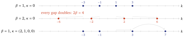
Proposition B.35 (An asymptotic Bethe ansatz, exactly). Put $I_j=\kappa_j+\tfrac12(N+1-2j)$ . Then $I_1>I_2>\dots>I_N$ lie in $\Z+\tfrac{N-1}2$ — the quantum numbers of Lecture 11, (11.11) — and $\kappa\mapsto I$ is a bijection onto the strictly decreasing sequences there that are bounded below by $-\tfrac{N-1}2$ . On a circle of circumference $L=\pi$ the momenta (B.32) are the unique solution in the ordered sector $k_1>\dots>k_N$ of $k_jL+\sum_{l\ne j}\varphi(k_j-k_l)=2\pi I_j, \qquad \varphi(k)=-\pi(\beta-1)\,\sgn k ,$ (B.33) that is, of Lecture 16’s unified logarithmic form (16.5) with a phase function that is a step. The ground state $\kappa=0$ is the symmetric block $I=\bigl(\tfrac{N-1}2,\dots,-\tfrac{N-1}2\bigr)$ , as it is for Lieb–Liniger.

Proof (★). In the ordered sector $\sum_{l\ne j}\sgn(k_j-k_l)=(N-j)-(j-1)=N+1-2j$ is fixed, so (B.33) reads $\pi k_j-\pi(\beta-1)(N+1-2j)=2\pi\kappa_j+\pi(N+1-2j)$ , which determines $k_j$ uniquely and gives (B.32); and those $k_j$ are ordered, since $k_j-k_{j+1}=2(\kappa_j-\kappa_{j+1})+2\beta\ge2\beta>0$ checked. The sector is a hypothesis, not a convenience: unlike Lecture 11’s increasing Lieb–Liniger phase, a step does not force the order of the roots from the order of the quantum numbers, and (B.33) can have further solutions outside the sector. At $N=2$ , $\beta=3$ , $I=(\tfrac12,-\tfrac12)$ the intended root is $(3,-3)$ , of energy $9$ ; $(-1,1)$ solves the same two equations, with energy $1$ . (At $N=2$ the reversed sector gives $k=(2-\beta,\beta-2)$ , consistent only for $\beta>2$ ; a spurious root needs a large enough $\beta$ , not merely $\beta>1$ .)

The normalisation of $\varphi$ is not free, and the check is Lecture 16’s. The kernel is $K=\varphi'=-2\pi(\beta-1)\delta$ , so the density equation (16.5) collapses to $\rho+\rho_h=\tfrac1{2\pi}-(\beta-1)\rho$ ; in the ground state $\rho_h=0$ and $\rho=1/2\pi\beta$ , the direct count, the $k_j$ being $2\beta$ apart in a box of length $\pi$ . The same momenta also solve (B.33) with the step $-\pi\beta\sgn k$ and $I_j=\kappa_j$ — Sutherland’s form, whose $\theta$ sits on the other side of the equation — but those quantum numbers are not distinct (in the ground state, all zero), so Lecture 16’s counting function, which wants one root per vacancy, does not apply, and substituting its kernel anyway returns $\rho=1/2\pi(1+\beta)$ checked. The two differ by the statistics phase $\pi\sgn k$ , and the course’s bookkeeping — distinct quantum numbers in $\Z+\tfrac{N-1}2$ , as in Lecture 11 — picks the first. Its vanishing at $\beta=1$ is Girardeau’s map again.

So the Bethe ansatz is present as an accounting identity and absent as a method. The scattering reading is Sutherland’s, and it belongs to the model on a line, where the same momentum-independent phase shift appears: a packet with non-zero relative momentum stays on one side of the step, so $\dd\varphi/\dd k=0$ there and Lecture 11’s dictionary row gives a vanishing time delay — the quantum form of Theorem B.22’s permuted momenta and no displacement cited: Sutherland (1971). On the circle there is no asymptotic region, and (B.33) is bookkeeping.

B.25 Dyson’s three ensembles

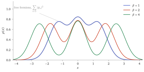
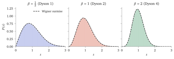
Remark B.36 (The ground state is a random-matrix ensemble). In the variable (B.31), $\abs{\psi_0^{\mathrm S}}^{2}\propto\prod_{i<j}\abs{z_i-z_j}^{2\beta}$ on the unit circle, which up to normalisation is the joint eigenvalue density of Dyson’s circular ensemble of index $2\beta$ cited: Dyson (1962); Mehta ch. 11. The three classical values $\beta=\tfrac12,1,2$ are the orthogonal, unitary and symplectic ensembles, Dyson’s $1,2,4$ — the three random-matrix ensembles of level statistics, appearing here as the positions of particles in a ground state (Figure B.15). The repulsion exponent is the Jastrow exponent: $P(s)\sim s^{2\beta}$ as $s\to0$ is the vanishing of $\psi_0^{\mathrm S}$ at a collision, squared.

Figure B.15. Nearest-neighbour spacings of the particle positions in the Sutherland ground state at

N=16

, sampled directly from

\abs{\psi_0^{\mathrm S}}^{2}

by Metropolis — no random matrix is diagonalised — against the Wigner surmises for Dyson index

2\beta

(dashed). The generator enforces agreement to

0.008

in distance between the distribution functions on a fixed grid, a fitted small-

s

exponent equal to

2\beta

within

0.3

, and the same distance, at

\beta=1

, to the spacings of an actual

\mathrm{CUE}

matrix.

B.26 What is shared with the Bethe ansatz, and what is not

Nothing in this lecture was an $R$ -matrix: no auxiliary space, no monodromy matrix, no $RTT$ relation, and Corollary B.15 is not $\{\,\dd^{k}\ln t(\lambda)\,\}$ for any $t$ — the tower of Lecture 15’s reading comes from one transfer matrix and one solution of the Yang–Baxter equation, while $I_k$ comes from $N$ operators that commute before anything is traced. Nor was there a Bethe ansatz: Proposition B.35 reports the answer in Bethe form rather than obtaining it. Both are claims about the route; the trigonometric model does carry a braid-group structure, Cherednik’s, and the next reading says where.

What is shared: infinitely many commuting charges, one of them the Hamiltonian; a many-body problem fixed by two-body data, one exponent $\beta$ per pair, with free particles at shifted momenta; and non-diffractive scattering (Lecture 12, Lecture 13) in the strongest form there is, the phase shift being constant. The difference is where the structure sits: in Lecture 14 and Lecture 15 in an algebra of operators on an auxiliary space, here in the symmetric group.

B.27 Creation operators, Cherednik’s operators, and exclusion statistics

Four continuations, each of which is a small subject.

What the charges are, and what they are not. $I_k$ of Corollary B.15 is a differential–difference operator of order $k$ involving every particle; it is not a sum of local densities of bounded range, and there is no lattice here for Definition 19.1 to apply to. The family is also not the one Theorem B.1 produced classically: $\tr L^{k}$ quantises to something with ordering ambiguities, and the Dunkl construction sidesteps that question rather than answering it. What is true is that the $I_k$ commute, that $I_2$ is the Hamiltonian, and that $N$ of them are algebraically independent — which is the count Liouville would have asked for cited: Polychronakos (1992).

Creation operators. Theorem B.16 gives the trapped spectrum but not a ladder: it produces eigenvalues by triangularity, not by raising a state. A ladder exists, and it lives in the gauge-transformed picture, which is the thing to get right. Put $a_i^{\pm}=\frac1{\sqrt{2\freq}}\bigl(\freq x_i\mp D_i\bigr) , \qquad \comm{a_i^{-}}{a_j^{+}}=\comm{D_i}{x_j}$ with (B.29) on the right: a deformed Heisenberg algebra whose deformation is made of transpositions. The symmetric combinations $B_k^{+}=\sum_i(a_i^{+})^{k}$ raise the energy by $k\freq$ , and the $N$ of them with $k=1,\dots,N$ generate the whole spectrum freely — but from the Gaussian $G=e^{-\freq\sum_jx_j^{2}/2}$ , not from $\psi_0^{\mathrm C}$ . The physical states are $\Delta^{\beta}B^{+}_{k_1}\cdots B^{+}_{k_r}G$ ; equivalently, the physical ladders are $\mathcal B^{+}_k=\Delta^{\beta}B^{+}_k\Delta^{-\beta}$ , applied to $\psi_0^{\mathrm C}$ cited: Brink, Hansson and Vasiliev (1992), eqs. (2), (4), (12); Polychronakos (1992). Applying the displayed $B_k^{+}$ to $\psi_0^{\mathrm C}$ itself leaves the Hilbert space: at $N=2$ , $\beta=\freq=1$ , $B_2^{+}\psi_0^{\mathrm C}$ acquires a $2/r^{2}$ and is not square-integrable. With the gauge right, the spectrum is that of $N$ independent bosonic modes of frequencies $\freq,2\freq,\dots,N\freq$ , so the multiplicity of $E_0+\freq n$ is the number of partitions of $n$ into parts of size at most $N$ — the conjugate of Theorem B.16’s count, and equal to it. That is also why the multiplicities do not depend on $\beta$ .

Cherednik’s operators. The $D_i$ of (B.11) are the rational Dunkl operators, and Theorem B.33 did not use them: the Sutherland model needed its own conjugation, done by hand. There is a trigonometric analogue, Cherednik’s: commuting first-order differential–difference operators in $z$ , built from $z_j\partial_{z_j}$ and the transpositions, whose algebra is the degenerate affine Hecke algebra — and that is where the braid relations hidden in this model live. Two distinctions are easy to lose. The individual Cherednik operators do not preserve the symmetric polynomials; their eigenfunctions are the non-symmetric Jack polynomials, and it is their symmetric combinations that act on $\Lambda^{\mathrm{sym}}$ and are diagonalised by the $J_\kappa$ of Theorem B.33. And the $q$ -difference theory, where $z_j\mapsto qz_j$ , is a different and larger story: it produces Macdonald polynomials and the double affine Hecke algebra, with the Jack polynomials recovered in a degeneration cited: Cherednik (1991); Macdonald §VI.10.

A discrepancy in the standard reference. Sutherland’s Beautiful Models §5.2.5 gives the trigonometric spectrum twice. Its first form, $E=(2\pi^{2}/L^{2})\bigl[\sum_jn_j^{2} +\lambda\sum_{j>i}\abs{n_j-n_i}\bigr]+E_0$ on a circle of circumference $L$ , is (B.32) exactly, with $\lambda=\beta$ , $n=\kappa$ , $L=\pi$ . The last line of the same equation, and the momenta of §5.2.6, print $k_j=(2\pi/L)[n_j+\lambda(N+1-2j)]$ — twice the shift, and inconsistent with the same book’s own $E_0=\pi^{2}\lambda^{2}N(N^{2}-1)/6L^{2}$ . The free-fermion case settles it: at $\lambda=1$ , $N=2$ , $L=\pi$ the ground state is $\sin(x_1-x_2)$ , whose momenta are $\pm1$ and whose energy is $1$ , which is that $E_0$ ; the printed momenta give $\pm2$ and $4$ . Replacing $\lambda$ by $\lambda/2$ in those two places repairs both checked; pages rendered, not extracted.

Fractional exclusion statistics. The density equation after Proposition B.35 reads $\rho_t=\tfrac1{2\pi}-(\beta-1)\rho$ : each root present removes $\beta-1$ vacancies beyond the one it occupies. Haldane read this as a statistics interpolating between bosons and fermions, with $\beta=1$ the fermionic point where nothing is removed. The thermodynamics is then a one-line modification of Lecture 17’s counting — the binomial coefficient $\binom{L\rho_t\dd\lambda}{L\rho\dd\lambda}$ of Proposition 17.4 acquires a $\beta$ -dependent number of slots — and reproduces the Calogero–Sutherland free energy cited: Haldane (1991); Wu (1994). It is the course’s cleanest example of a delta-function kernel: Lecture 16’s integral equation becomes local in momentum, and the thermodynamics is algebra rather than an integral equation.

B.28 The frontier, and reduction as a construction principle

Four directions lead out of this course. Classification. Which $\Rmat(\bethe)$ solve the Yang–Baxter equation? Classically there is a theorem: Belavin and Drinfeld sorted the non-degenerate solutions of (14.12) for a simple Lie algebra into rational, trigonometric and elliptic families. Quantum mechanically no list is closed, even for a two-dimensional auxiliary space and even of difference form, and the Hubbard model’s $\Rmat$ (optional lecture C) is of no difference form at all. The systematic language is quantum groups: Yangians and affine quantum algebras, whose representations are the $\Rmat$ -matrices. Separation of variables. Sklyanin’s method replaces the Bethe ansatz by a change of variables to the eigenvalues of $B(\bethe)$ — and on the homogeneous chain $B$ lowers $S^{z}$ by one, so it is nilpotent and there are none to change to, and the construction must twist the monodromy first. (The pseudovacuum was never the problem: Lecture 15 built it.) It is where the spectral curve $\det(z-\mono(\bethe))$ of Lecture 9’s reading returns, as a quantum spectral curve. Beyond Euler. Equation (20.5) is the leading order; diffusive corrections, and the anomalous transport of the isotropic Heisenberg chain, are current work. Integrable circuits. Discrete-time quantum circuits built from solutions of Yang–Baxter are integrable models in which everything here can be recomputed, and are the form in which the subject has reached quantum simulators.

And one principle. This lecture built the Calogero–Moser system out of free motion on $\Herm(N)$ , a symmetry, a moment-map constraint and a gauge fixing. Reduction returns in three places, all of them beyond this course.

Quantum Hamiltonian reduction. The classical recipe has an operator version: free motion becomes the Laplacian on a group, the constraint becomes a representation-theoretic condition, and the radial part of the Laplacian is the Calogero–Sutherland operator of §B.21. This is why the Dunkl operators of §B.7 look like covariant derivatives: they are.

Nested systems from root systems. The Calogero–Moser models are indexed by root systems (§B.19), and so are the nested Bethe equations of optional lecture C, by the Cartan matrix of the same diagram.

Spectral curves. The curve of §9.13 (Lecture 9’s reading) is a reduction too, of a much larger linear problem, and the modern statement — that integrable systems of this type are classified by moduli of curves with data on them — is the subject that reading’s pointer was aiming at.

What all three share is the shape of Theorem B.8: a free system, a symmetry, a constraint and a choice of gauge. It is worth carrying out of the course as a question to ask of any solvable model — what is it a reduction of?

B.29 Two by two

Everything in this lecture can be seen for $N=2$ , in the coordinates $X=q_c\Id+\mathbf x\cdot\boldsymbol\sigma$ of Example B.4.

Orbits. The orbit of a regular $X$ is the sphere $\abs{\mathbf x}=r$ at fixed $q_c$ , of dimension $2=4-2$ (Proposition B.24); conjugation rotates $\mathbf x$ , and the stabiliser rotates about the axis through $\mathbf x$ (Figure B.16). A degenerate $X=q_c\Id$ is its own orbit, a single point, with all of $\U(2)$ as stabiliser: the bigger the stabiliser, the smaller the orbit, $\dim(\text{orbit})=\dim G-\dim(\text{stabiliser})$ .

The momentum map. $\comm{\mathbf x\cdot\boldsymbol\sigma}{\mathbf v\cdot\boldsymbol\sigma}=2\ii(\mathbf x\times\mathbf v)\cdot\boldsymbol\sigma$ , so $\momap=2\ii\boldsymbol\ell\cdot\boldsymbol\sigma$ and $\xi=\ii g\sigma_1$ is $\boldsymbol\ell=(g/2,0,0)$ . Its stabiliser is $\{U:Ue\propto e\}$ , the unitaries diagonal in the eigenbasis of $\sigma_1$ : rotations about the $\ell$ -axis, $\U(1)\times\U(1)$ , of dimension $2=1+(N-1)^{2}$ . The orbit of $\xi$ is the sphere $\abs{\boldsymbol\ell}=g/2$ , of dimension $2N-2=2$ (Proposition B.6).

The reduction. $8=2N^{2}$ dimensions; the constraint fixes the three components of $\boldsymbol\ell$ , leaving $5$ ; the residual rotations about $\boldsymbol\ell$ remove $1$ , leaving $4=2N$ : centre of mass, gap, and their momenta. Gauge-fixing $\mathbf x$ onto the $\sigma_3$ axis makes $X$ diagonal, and the constraint then forces $\mathbf v$ ’s $\sigma_2$ -component to carry the angular momentum: $P_{12}=\ii g/(q_1-q_2)$ .

Figure B.16. An orbit of conjugation,

N=2

, at fixed trace. Hermitian matrices with eigenvalues

q_c\pm r

form a sphere of radius

r

; the diagonal ones are its two poles on the

\sigma_3

axis. The stabiliser of a point acts as the rotations about the axis through it (with the scalars, the unitaries diagonal in a basis where the point is diagonal). The centre,

r=0

, is an orbit on its own.

B.30 Two particles, done by hand

Everything in this lecture is visible at $N=2$ , where no symmetric-function theory is needed. Separate the centre of mass $R=(x_1+x_2)/2$ and the relative coordinate $r=x_2-x_1>0$ on the chamber. Then $-\tfrac12(\partial_1^{2}+\partial_2^{2})=-\tfrac14\partial_R^{2} -\partial_r^{2}$ and $\tfrac12\freq^{2}(x_1^{2}+x_2^{2}) =\freq^{2}R^{2}+\tfrac14\freq^{2}r^{2}$ , so (B.8) splits into an oscillator in $R$ , of levels $\freq(n_{\mathrm{cm}}+\tfrac12)$ , and $h_{\mathrm{rel}}=-\partial_r^{2}+\frac{\beta(\beta-1)}{r^{2}} +\frac{\freq^{2}}4r^{2},$ whose eigenfunctions are $r^{\beta}e^{-\freq r^{2}/4}$ times Laguerre polynomials in $\freq r^{2}/2$ and whose levels are $\freq(2n+\beta+\tfrac12)$ . Five things to check, in this order.

(a) The ground state and the spectrum. The product of the two ground states is $r^{\beta}e^{-\freq(2R^{2}+r^{2}/2)/2}$ , which is (B.9) at $N=2$ , with $E_0=\freq(\tfrac12+\beta+\tfrac12)=\freq(1+\beta)$ , matching (B.10). The full spectrum is $E_0+\freq(n_{\mathrm{cm}}+2n)$ , and the number of ways to write $k$ as $n_{\mathrm{cm}}+2n$ is $\lfloor k/2\rfloor+1$ , the partitions of $k$ into at most two parts. Theorem B.16 at $N=2$ , obtained without a single Dunkl operator — and, unlike the theorem, with completeness thrown in, since the radial problem’s eigenfunctions are a known complete set. A finite-difference diagonalisation of $h_{\mathrm{rel}}$ confirms the levels and finds nothing between them.

(b) The domain is doing work. The other indicial root gives $r^{1-\beta}e^{-\freq r^{2}/4}$ , also positive, also a solution, with the lower value $\freq(\tfrac32-\beta)$ . For $\beta\ge\tfrac32$ it is not square-integrable — at $\beta=\tfrac32$ exactly, $r^{-1}$ diverges logarithmically — and the question does not arise; for $\tfrac12<\beta<\tfrac32$ it is, and it belongs to a different self-adjoint operator — one of the family Definition B.30 chooses among. At the endpoint $\beta=\tfrac12$ the two exponents coincide, the second solution is $r^{1/2}\ln r$ , and the two values are equal: there is nothing to choose between. This is Remark B.31 in one dimension, and it is the reason Definition B.30 comes before Theorem B.11. For $N\ge3$ the partner fails earlier than $\beta=\tfrac32$ , at the total collision; Remark B.31 says where.

(c) The Dunkl algebra. With $s=s_{12}$ , $D_1=\partial_1-\beta(1-s)/r$ and $D_2=\partial_2+\beta(1-s)/r$ . Verify on $f=x_1^{2}$ that $D_1f$ and $D_2f$ are polynomials and that $D_1D_2f=D_2D_1f$ . Then check that $D_1$ is not a derivation — the trap of Definition B.12: $D_1(x_1x_2^{2})-(D_1x_1)\,x_2^{2}-x_1\,D_1(x_2^{2}) =\beta\,(x_1-x_2)(x_1+x_2)\ne0 ,$ (B.34) from $D_1x_1=1+\beta$ , $D_1(x_2^{2})=-\beta(x_1+x_2)$ and $D_1(x_1x_2^{2})=x_2^{2}-\beta x_1x_2$ . Then take $f$ symmetric, check $D_if=\partial_if$ , and rediscover (B.12): $-\tfrac12\sum D_i^{2}f=-\tfrac12\sum\partial_i^{2}f +\beta(\partial_1f-\partial_2f)/r$ . At $N=3$ the same calculation on $f=x_1^{2}$ gives $\comm{D_1}{D_2}f=0$ in four lines, and is the smallest case in which the three-index terms of Theorem B.13 appear at all.

(d) Bohr–Sommerfeld, exactly. For $A>0$ and $E>\freq\sqrt A$ the classical orbit of $h_{\mathrm{rel}}$ with coupling $A$ has two turning points and action $\oint p\,\dd r/2\pi=(E/\freq-\sqrt A)/2$ , so $I=n+\tfrac12$ gives $E=\freq(2n+1+\sqrt A)$ . That is the exact level $\freq(2n+\beta+\tfrac12)$ if and only if $\sqrt A=\beta-\tfrac12$ : the Langer value $A=(\beta-\tfrac12)^{2}$ , not the bare $A=\beta(\beta-1)$ . Comparing the two needs $\beta>1$ , where the bare coupling is positive; for $\tfrac12\le\beta<1$ it is negative, the classical particle falls into the collision and the bare action diverges, while the Langer-corrected rule still returns the exact levels. Where the comparison is legitimate the bare rule is wrong by $\freq\bigl(\beta-\tfrac12-\sqrt{\beta(\beta-1)}\bigr)$ , a constant that does not shrink at large quantum numbers checked. The Bohr–Sommerfeld rule of Lecture 6’s reading is therefore exact here in the sense semiclassics always means it, and this is the cheapest place in the course to see what the Langer correction is for.

(e) Sutherland at $N=2$ . On the circle, $\psi_0^{\mathrm S}=\sin^{\beta}r$ and $E_0^{\mathrm S}=\beta^{2}\cdot2\cdot3/6=\beta^{2}$ ; and (B.32) gives $k_{1,2}=2\kappa_{1,2}\pm\beta$ , so $E_\kappa=\tfrac12\bigl[(2\kappa_1+\beta)^{2}+(2\kappa_2-\beta)^{2}\bigr]$ . At $\beta=1$ , $\kappa=0$ , that is $E=1$ with momenta $\pm1$ : the two impenetrable bosons of Girardeau’s map (Lecture 18’s reading), which are one antiperiodic fermion pair. The formal value $\beta=0$ gives free bosons at rest, $E=0$ — the one exponent at which the shift disappears, and the only one at which the ground state is not an ensemble. It lies outside Definition B.30’s $\beta\ge\tfrac12$ , being the partner of $\beta=1$ .

Calogero–Moser, classical and quantum

What this lecture does

B.1 The question

B.2 The model, and Moser’s Lax pair

B.3 Free motion in disguise

B.4 A conserved commutator, and a level with no collisions

B.5 The reduction: Moser’s $L$ is the free momentum

B.6 The quantum gas, and its Jastrow ground state

B.7 Dunkl operators

B.8 The trapped spectrum, and isochrony

B.9 What it buys

B.10 Caveats, in one place

B.11 Moser’s Lax pair, derived

B.12 Independence

B.13 Involution, and the dynamical $\rmat$ -matrix

B.14 Scattering, and the comparison with Toda

B.15 The trapped Lax pair

B.16 The projection theorem, proved

B.17 Conjugation, its momentum map, and the reduction theorem

B.18 Regular and singular levels

B.19 Root systems and the other Calogero–Moser models

B.20 Ruijsenaars–Schneider

B.21 The quantum models, carefully: units, the circle, the domain

Why it is the ground state, and why positivity is not the reason

B.22 The trapped spectrum, drawn

B.23 The Jastrow computation, and Dunkl’s two theorems

B.24 Sutherland’s excited states

Free fermions with shifted momenta

B.25 Dyson’s three ensembles

B.26 What is shared with the Bethe ansatz, and what is not

B.27 Creation operators, Cherednik’s operators, and exclusion statistics

B.28 The frontier, and reduction as a construction principle

B.29 Two by two

B.30 Two particles, done by hand

Summary

References

B.1 The question

B.2 The model, and Moser’s Lax pair

B.3 Free motion in disguise

B.4 A conserved commutator, and a level with no collisions

B.5 The reduction: Moser’s LLL is the free momentum

B.6 The quantum gas, and its Jastrow ground state

B.7 Dunkl operators

B.8 The trapped spectrum, and isochrony

B.9 What it buys

B.10 Caveats, in one place

B.11 Moser’s Lax pair, derived

B.12 Independence

B.13 Involution, and the dynamical r\rmatr-matrix

B.14 Scattering, and the comparison with Toda

B.15 The trapped Lax pair

B.16 The projection theorem, proved

B.17 Conjugation, its momentum map, and the reduction theorem

B.18 Regular and singular levels

B.19 Root systems and the other Calogero–Moser models

B.20 Ruijsenaars–Schneider

B.21 The quantum models, carefully: units, the circle, the domain

Why it is the ground state, and why positivity is not the reason

B.22 The trapped spectrum, drawn

B.23 The Jastrow computation, and Dunkl’s two theorems

B.24 Sutherland’s excited states

Free fermions with shifted momenta

B.25 Dyson’s three ensembles

B.26 What is shared with the Bethe ansatz, and what is not

B.27 Creation operators, Cherednik’s operators, and exclusion statistics

B.28 The frontier, and reduction as a construction principle

B.29 Two by two

B.30 Two particles, done by hand

Summary

References

B.5 The reduction: Moser’s $L$ is the free momentum

B.13 Involution, and the dynamical $\rmat$ -matrix

References

J. Moser, Adv. Math. 16 (1975) 197; F. Calogero, J. Math. Phys. 12 (1971) 419; Perelomov, Integrable Systems of Classical Mechanics and Lie Algebras, §§3.1, 3.3; J. Avan and M. Talon, Phys. Lett. B 303 (1993) 33; D. Kazhdan, B. Kostant and S. Sternberg, Comm. Pure Appl. Math. 31 (1978) 481; C. F. Dunkl, Trans. Amer. Math. Soc. 311 (1989) 167; Reed and Simon II, §X.1. The readings name their own sources.