C.1 The question
Lecture 13 gave labelled particles a matrix S-matrix and the Yang–Baxter equation. So the question is
how is a gas of particles with a spin quantised on a ring, when the two-body S-matrix is a matrix?
The answer: the ring condition is an eigenvalue problem for an inhomogeneous Heisenberg chain whose sites are the particles (Theorem C.2 and Proposition C.4), and its algebraic Bethe ansatz gives two coupled families of Bethe equations (Theorem C.6). The worked example is two particles (Example C.7).
C.2 Fermions with a spin, and a matrix S-matrix
The model is Lecture 11’s delta gas with one addition: each particle carries a spin- label, and the particles are fermions. On a ring of circumference , (C.1) acting on wavefunctions , , that are totally antisymmetric under exchanging a position and its label together. This is the Yang–Gaudin model (Yang 1967, Gaudin 1967). Write for the number of down spins, so , and take .
Remark C.1 (Units, and two names used twice). Units are Lecture 11’s, . The Hubbard hopping is a number, the transfer matrix always carries its argument; the Hubbard is a spin rapidity, Lecture 15’s eigenvalue always carries its argument.
The two-body problem is two problems
Lecture 13 did the two-body problem for labelled particles. On write (C.2) with slot of the tensor holding the label of the particle at position , and extend by antisymmetry. Proposition 13.1 gives with (C.3) the permutation of the two label factors (Definition 9.4) and the projectors on labels symmetric and antisymmetric checked.
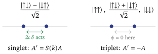
(C.3) is the whole reason this lecture exists. On the singlet — labels antisymmetric, positions symmetric — the delta acts and the amplitude picks up Lecture 11’s scalar . On the triplet the wavefunction vanishes where the particles meet, the delta never sees them, and the amplitude picks up (Figure C.1). One two-body problem, two answers; a scalar Bethe equation cannot hold both.
Following the momenta
Lecture 13 also fixed the object to work with. is written in the order of positions; the natural bookkeeping for a scattering problem follows the momenta, and there the two-body matrix is (Equation (13.3)), for fermions (C.4) with the course’s rational R-matrix and the Heisenberg Lax operator of Lecture 14. We drop the subscript : in this lecture always means the fermionic one. Three facts, all checked symbolically, carry the lecture: (C.5) The last is the Yang–Baxter equation (§13.3); the first is the only place a sign will come from in §C.3. Note that (C.4) uses , not : in the course’s ordering (Theorem 14.2) the Lax operator paired with is .
C.3 Periodicity is an eigenvalue problem
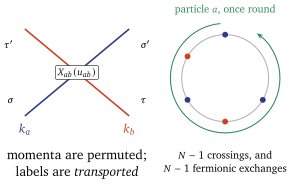
Inside the region the Bethe ansatz reads (C.6) slot of holding the label of the particle at position ; total antisymmetry then determines everywhere. The contact conditions at are Lecture 13’s walls, (Equation (13.5)), and in the momentum-ordered amplitudes of Lemma 13.2 they become (C.7) Each crossing of momentum lines and multiplies by (Figure C.2). Nothing is left to choose: the interaction has been used up. What remains is the ring.
Theorem C.2 (Periodicity). Let be pairwise distinct, no two differing by (so that every is defined), and let be the totally antisymmetric extension of (C.6) with amplitudes satisfying (C.7). Then is periodic in every variable if and only if, for every and , (C.8) These conditions are equivalent to conditions on a single vector sketched here; proved in the reading below, (C.9) every factor at its own argument .
Proof. Because is antisymmetric, periodicity in one argument at every configuration gives it in all of them; take the first. Let and shift by . The shifted point has its arguments in the order , so moving the first argument past the other costs : and both sides of are now values of (C.6). Matching the coefficient of each plane wave: the term on the right contributes and the momentum word , while the slots of are read in the cyclic order . Writing for the cycle , , and for the operator that permutes slots that way, the condition is (C.10) Now pass to . Since is a homomorphism, , so and the relabelling operator cancels: (C.10) is . The permutation is with its momentum word shifted one place left, reached from by , and at each step (C.7) applies with first leg throughout: . That is (C.8).
The conditions for different reduce to (C.9): those with the same are conjugate by the Yang–Baxter equation, and a chain of the ’s carries the others onto (below).
Proof of the reduction, and the two places it can go wrong (★). Same . If with , so that and share and differ by exchanging two letters of the word, then , and the Yang–Baxter equation (C.5) in the form (C.11) conjugates the whole product: the operator in (C.8) for is times the one for times , because the remaining factors with have legs disjoint from . So the two conditions are the same condition. The order in (C.11) matters: with the two exchanged the identity is false, and at with the two sides differ by an exact rational in the largest entry checked.
Different . Every with is therefore equivalent to the cyclic word , with ; but that is a condition on , not on . They are the same condition, by an induction on . The word is with its first letter moved to the back, reached by , and the crossings accumulated on the way are exactly , so (C.12) If the condition for holds, acts on as the non-zero scalar , so is a non-zero multiple of . Starting from , every is a multiple of and the conditions are (C.9); conversely (C.12) runs the same induction backwards. All conditions, and the chain, are verified at and checked.
The fermionic sign in (C.9) is not cosmetic: at dropping it changes to , and moves the root by a factor at , checked.
The product of crossings is a transfer matrix
(C.9) is eigenvalue problems for different operators, which looks hopeless. It is not: the operators are values of one commuting family, and it is a family we have already solved.
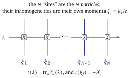
Definition C.3 (The auxiliary chain). For momenta as in Theorem C.2, put , adjoin an auxiliary labelled , and set (C.13)
Its quantum spaces are the labels of the particles, its “sites” the particles themselves, at inhomogeneities equal to their own momenta: no lattice, no spin Hamiltonian, a bookkeeping device that happens to be integrable.
Proposition C.4 (The crossings are the transfer matrix). For every , .
Proof. At the th factor of (C.13) is : Push to the right using for ; the factors to the right of it become operators on the quantum spaces alone, , which involves only the spaces and so commutes with . Hence , and , valid for any not acting on space , gives .
Proposition C.5 (The chain is Heisenberg). : the auxiliary chain is an inhomogeneous Heisenberg chain, up to one scalar. Consequently and for all away from the poles .
Proof. The displayed identity is (C.4) factor by factor. The relation (Theorem 14.2) needs only that every site operator obeys with one common , and the shifts cancel in the argument of , , so commutativity follows as in Theorem 14.3; scalars commute with everything checked.
So all conditions can be imposed at once: ask for a common eigenvector of the family and read off the numbers . This is the whole of nesting. The first Bethe ansatz reduced the gas to a finite linear-algebra problem in the labels; the second solves that problem.
C.4 The nested Bethe equations
Lecture 15 solved this chain for equal inhomogeneities, and nothing in the solution used that they are equal: with at site the relation holds as before (Theorem 14.2 needs only a common ), the exchange relations are unchanged, and the reference-state eigenvalues (15.4) become and checked, . Work with the unnormalised monodromy of Proposition C.5, (C.14) whose entries are the below — not those of (C.13), which differ from them by the scalar and would give . Its reference state is all labels up, , on which is triangular with and ; creates; and for pairwise distinct , none equal to or , the vector is an eigenvector of the whole family, with (C.15) provided the residues at cancel (Corollary 15.9).
The spin rapidities below are , minus Lecture 10’s convention; for generic inhomogeneities the mirrored roots do not solve the spin equations, and the reading at the end of this lecture says why the sign is not free.
Theorem C.6 (The nested Bethe equations, Yang and Gaudin 1967 proved, given the reduction of Theorem C.2, sketched here). Let be pairwise distinct with no two differing by (so that no in (C.9) is singular), let be pairwise distinct and (Corollary 15.9’s regular roots, ), put , and let Then , if it is not zero, satisfies every periodicity condition (C.9), and the resulting eigenfunction of (C.1) has (C.18)
Proof. (C.17) is Corollary 15.9’s system (15.17) for the inhomogeneous chain, written in : the residue of (C.15) at vanishes exactly when . So is a common eigenvector and Proposition C.4 turns (C.9) into scalar equations, , with the eigenvalue of (C.13). Evaluate it. By Proposition C.5, ; at the second term of (C.15) carries the factor and dies, and the first term’s prefactor cancels the denominator exactly, leaving (C.19) Then for every , and what is left is (C.16). Inside the sectors every term of (C.6) is a plane wave of energy and momentum , as in Theorem 11.3.
The two sets do different jobs. The are momenta and carry the energy (C.18). The are dimensionless, as many as there are down spins, and carry none of it — they enter (C.16) only as phase shifts. That is spin–charge separation in its rawest form (a reading draws two states).
The counting. In logarithms, (C.20) with and , and . The parities are part of the equations: a wrong one solves (C.16) with an extra minus sign, invisible in (C.20) checked.
Example C.7 (: the two channels, again). Take , . (C.17) reads , whose only root is ; then and (C.16) becomes exactly Lecture 11’s Lieb–Liniger equation (11.9) for two particles. The other state is the descendant , where the right-hand side of (C.16) tends to : free fermions. The two channels of Figure C.1, recovered from the nesting checked.
Whether these solutions exhaust the spectrum is a separate question, and the answer is Lecture 10’s reading’s for the Heisenberg chain: they do not, without the complex ones. The reading at the end says what is known cited: Takahashi ch. 12; Essler et al. ch. 4.
C.5 The Hubbard model
The Hubbard model’s Bethe equations are stated here, and their derivation cited; the tutorial solves the lattice two-body problem, which fixes the correspondence with §C.4, sign included.
On a ring of sites, even, with creating an electron of spin at site and , (C.21) and we set : the Yang–Gaudin gas put on a lattice, with the dispersion , which is not quadratic, so there is no Galilean invariance.
Theorem C.8 (Lieb and Wu 1968). The regular eigenstates of (C.21) with electrons and down spins — those with finite, pairwise distinct roots, and — are given by charge momenta and spin rapidities solving with cited: Lieb and Wu (1968); Essler et al. ch. 3. They are not all the states, and not all the rest are symmetry descendants either (the reading gives one of each on a six-site ring).
With they are (C.16)–(C.17) under (C.24) with that sign: with none of the eighteen singlet states of the two-electron ring satisfies (C.22); with it, all do checked. Shastry’s -matrix behind them is not of difference form, which Lecture 14 and Lecture 15 used (the reading). For species the construction nests times, one level per node of the Dynkin diagram (the reading).
Elastic non-diffractive scattering: the asymptotic momenta are only permuted, and a collision leaves a displacement (Theorem 12.2, cited)⟶the momenta are still only permuted ((C.18)) and a collision still leaves a phase, but the labels are transported by (Figure C.2), so the ring condition is an eigenvalue problem and not a number (type A; the Part II side proved, the Part I side cited)
C.6 What it buys
Nesting: a matrix S-matrix on a ring is an eigenvalue problem, and the eigenvalue problem is an inhomogeneous Heisenberg chain whose sites are the particles (Propositions C.4 and C.5), so the algebraic Bethe ansatz solves it.
Two families of rapidities: the momenta carry all of the energy, the spin rapidities none of it (Theorem C.6).
The Hubbard model’s equations, the same system under , (Theorem C.8, cited).
C.7 Caveats, in one place
Status. Theorem C.2 is proved, except that its reduction of the conditions to on one vector is sketched here and proved in a reading; Propositions C.4 and C.5 are proved; Theorem C.6 is proved given that reduction and the algebraic Bethe ansatz of Lecture 15 with unequal inhomogeneities, checked here at . The Lieb–Wu equations are cited; their case is derived in the tutorial.
Completeness is not claimed, for the gas or for the lattice: the nested equations need complex spin roots, and the regular Lieb–Wu solutions miss states (the readings).
The fermionic sign and the Hubbard sign are not conventions; each wrong choice gives wrong numbers.
C.8 The auxiliary chain drawn; which shift; two states drawn
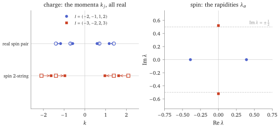
Remark C.9 (Which shift, and why it is not free). Write the spin rapidities as . Lecture 15’s homogeneous chain names the same roots ((15.6)), so this lecture’s is minus Lecture 10’s. There the sign was a labelling: the homogeneous system is invariant under and the two choices name a mirror doublet, which only the vector tells apart. Here the ambiguity generically does not arise — for generic inhomogeneities the spin equations are not invariant and the mirrored roots do not solve them, although a symmetric set such as is invariant (at both roots solve it) — but the check script builds anyway and confirms it is the eigenvector used checked.
scripts/figures/nested_roots.py.C.9 The Hubbard model’s symmetry, and a check
The equations of Theorem C.8 are checked against exact diagonalisation of a six-site ring, where of the states of the singlet sector are regular Bethe states and the twenty-first is the -pair of Remark C.10. Eighteen of the twenty — those with , complex roots included — are checked to by reconstructing the roots from ; that reconstruction degenerates at , so the two states there are checked directly against the equations instead checked. The commutators below are computed exactly, on one even ring; they are why is even.
Remark C.10 (). (C.21) has more symmetry than the spin . Let create a pair on a site, with the staggering. Then all three for even : the hopping terms cancel in pairs along the ring, and the closing bond cancels only if . At , the commutator misses by checked. So carries a second commuting with the first. As Lie algebras ; the of the familiar statement lives at the group level, and no commutator can see it.
For the printed the ’s are spectrum-generating, not symmetries: moves the energy rather than fixing it, and it is whose degeneracies organises cited: Yang (1989); Essler et al. ch. 2. The staggering makes anticommute with the translation, so it raises the momentum by , and is an exact eigenstate of (C.21) of energy at checked — and outside Theorem C.8, because at every finite Bethe pair has , so , while exact diagonalisation at returns and .
C.10 Higher rank: where the Dynkin diagram comes in
Nothing in §C.3 used that the label space is . For species the two-body matrix is still with on , it still obeys the Yang–Baxter equation checked, and Theorem C.2 and Proposition C.4 go through word for word. What changes is §C.4. The auxiliary monodromy is now in the auxiliary index — the transfer matrix still acts on the -dimensional label space — its reference state breaks to , and its first row carries creation operators in place of Lecture 15’s single . A Bethe vector therefore carries a vector of indices, and choosing that vector is itself a Bethe-ansatz problem of rank , whose auxiliary problem needs another, and so on — levels, the last of them scalar. That is why the procedure is called nesting, and the extra creation operators are what Lecture 15’s reading pointed at.
The bookkeeping is the Lie algebra’s. commutes with for every checked, so the hierarchy is -invariant, and the levels are the nodes of the Dynkin diagram : level carries rapidities , and the equations couple level to level through the Cartan matrix, (C.25) the source appearing only at the node the particles attach to — the left-hand side is at every other node, — and the term excluded: with it would contribute and turn the case into checked. Equation (C.17) is that case (Figure C.5); the pair, whose second equation contains no at all, is in the reading cited: Sutherland (1968), (16)–(17); Babelon, de Vega and Viallet (1982).
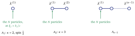
The same diagram indexes the other series once the label space carries a different representation, and then the representation data — weights, matrix elements of the generators — is what the computation needs; the rep-engine package supplies it exactly, and the check script takes ’s fundamental from it.
In the reading of optional lecture B the root systems , , , index classical Calogero–Moser models, one interaction per positive root; here indexes the levels of a quantum Bethe ansatz, one set of rapidities per node. The same combinatorial object, two unrelated uses, and no theorem in this course connecting them.
The root system of , indexing the classical Calogero–Moser models — one pair interaction per positive root (optional lecture B, reading)⟶the Dynkin diagram of , indexing the levels of the nested Bethe ansatz for -component particles — one set of rapidities per node, coupled by the Cartan matrix (C.25) (type A, cited)
C.11 Shastry’s R-matrix, and two transcription traps
The R-matrix. Shastry (1986) built a two-dimensional vertex model whose transfer matrix commutes with (C.21), by taking two six-vertex models at their free-fermion point and coupling them with a local diagonal factor whose parameter is tied to the spectral one by . Two things are worth separating. Jordan–Wigner is the transformation between the fermions and the spin variables, not the coupling. And the loss of difference form is not what stops at a special point from being the shift operator: that is regularity, , which Shastry’s matrix has. What difference form buys is one generating a whole commuting family from a single argument, which is what Lecture 14’s construction used cited: Shastry (1986); Essler et al. ch. 12.
The other nodes. For the second node of (C.25) reads with no in it at all: the second level sees the particles only through the first. Sutherland’s original writes both levels with an external minus and the self-root included, which is the same equation once the self-factor is taken across cited: Sutherland (1968), (16)–(17).
The two statistics. The bosonic of Lecture 13 also has , because : the two statistics are told apart by , not by the value at the origin, and Proposition C.4 holds for both. What they do not share is the periodicity condition checked.
An exceptional state. Theorem C.8 is restricted to regular solutions, and its escape clause is not decorative. At , , the symmetric wavefunction with is an exact eigenstate of energy at . Any two-root representation of it must satisfy , which here forces : at coincident roots the cusp condition gives and the ordinary ansatz vanishes, so this state is a regularised limit of a colliding pair, reached as along . Nor is it a descendant: annihilates it and the spin generators preserve the total spin checked.
The Hamiltonian. The reference book writes (C.21) in its particle–hole symmetric form, , so its energy carries an extra ; its coupling is , ours is written out; and its spin equation is the reciprocal of (C.23). All three differences are invisible in a formula copied out of context checked.
The gap. §C.12’s is the chemical-potential discontinuity. The same book’s is the single-holon threshold, exactly half of it, and is printed in Bessel form with . Which gap is meant is not a detail: the two differ by a factor of two at every coupling checked.
C.12 Half filling, the Mott gap, and spin–charge separation
At half filling, , the Hubbard model is an insulator for every . Lieb and Wu’s own paper established it from (C.22)–(C.23) in the thermodynamic limit: the charge gap, meaning the discontinuity of the chemical potential, is positive for every , tending to from above and to as cited: Lieb and Wu (1968), (21)–(23). Say which gap. The reference book’s (its (7.18)) is the single-holon threshold, exactly half of this, and is written in Bessel form with ; the two agree to every digit once converted checked. There is no metal–insulator transition at finite in one dimension; the transition is at . The spin sector meanwhile stays gapless, and at large the half-filled model reduces to the Heisenberg antiferromagnet of Lecture 10 with : second-order hopping of an electron onto an occupied site and back costs and gains , and it can only happen if the two spins are antiparallel. On a four-site ring, where the Heisenberg ground energy is , the two agree to at and at checked.
That is spin–charge separation, and it is visible already in §C.4: the energy (C.18) does not contain . In the thermodynamic limit the two sectors acquire different sound velocities — from the ’s and from the ’s — and an added electron’s charge and spin propagate apart. The Luttinger-liquid description of the resulting low-energy theory, and the angle-resolved photoemission experiments on quasi-one-dimensional conductors that look for the two dispersing features, are the obvious continuation cited: Essler et al. ch. 8; Giamarchi, Quantum Physics in One Dimension.
C.13 What is not claimed about the gas
That the solutions of (C.16)–(C.17) exhaust the spectrum is not proved here, and the situation is the one Lecture 10’s reading (§10.10) described for the Heisenberg chain: real roots do not suffice. Here the complex ones live in the spin sector — strings of ’s, one of which is drawn in Figure C.4 — while for the momenta stay real. Proposition 11.4 proves that for the spinless gas; for the spinful one it is Yang’s and Gaudin’s statement, and it is not proved here. Completeness is a counting statement with known exceptions cited: Takahashi ch. 12; Essler et al. ch. 4. The thermodynamics built on that string hypothesis — the analogue of Lecture 17 for two coupled families — is a genuine subject and is not attempted.
C.14 Bosons with a label, and the attractive gas
Two variants cost one line each and are worth knowing.
Two-component bosons. (C.3) becomes , so — the R-matrix itself rather than , and the interacting channel is now the symmetric one. The auxiliary chain is again of Heisenberg type, the fermionic of (C.9) is absent, and the nested equations come out with the shifts reflected. Substituting the bosonic into the fermionic condition without touching the statistics sign gives in the singlet: antiperiodic quantisation, and a spectrum wrong by half a level checked.
Attraction. For the need no longer be real (Proposition 11.4 assumed ), and the gas forms bound pairs of one up and one down spin — the one-dimensional analogue of a Cooper pair. In the thermodynamic limit the pair is the string cited: Gaudin, The Bethe Wavefunction, §11.4, where the string is presented as a large-system approximation. It is not exact on a finite ring: at , , the even bound wave is with , so ; at , the true is against the string’s checked. Nothing in §C.3 used the sign of ; everything in §C.4 about real solutions did.
C.15 Two electrons on a lattice, from scratch
The Lieb–Wu equations were stated, not derived. Here is the case in full, on a lattice of sites, and it is enough to fix (C.24) including its sign.
Take one up electron and one down electron; the spin singlet has a symmetric spatial wavefunction . For put set there and elsewhere. Away from the diagonal the lattice Schrödinger equation is free and gives for any .
The diagonal. At the equation reads and by symmetry and , while the free equation for continued to the diagonal is the same expression with every replaced by and no . Subtracting, Every term carries ; cancelling it leaves a linear relation whose coefficients are, with , checked. That is Lecture 11’s with and — (C.24), and its sign, derived rather than transcribed.
The ring. Periodicity relates the two amplitudes once more, and here it is worth doing rather than quoting: the antisymmetry sign of Theorem C.2 does not appear, because we are working with the symmetric spatial function of the singlet. Since , , so ; matching the coefficients of and gives which is (C.22) at once (C.23) has been used: at its right-hand side is and its left-hand side forces , so and the two displayed forms agree. Multiplying the two charge equations gives : the total momentum is quantised, as it must be.
The test. Diagonalise (C.21) on with one up and one down electron — a matrix — and resolve it by total momentum and by spatial symmetry. There are symmetric states. Eighteen of them, all those with , satisfy the displayed equation to at , and ; some need complex with , which is what a bound – pair looks like checked. The other three sit at , where the energy vanishes for every finite pair with and so cannot fix : there the equation has to be read directly. It gives , because makes and the ratio , so lies on the antiperiodic grid — the pairs with and with , which are the two states and are perfectly regular solutions checked; only the route to them fails. It is not true that any real pair summing to solves it: gives against . The third state, at , is the -pair of Remark C.10 and is outside Theorem C.8 altogether.
The continuum check, for comparison. Example C.7’s gas can be solved without any Bethe ansatz. At zero total momentum, , the relative coordinate obeys on a circle of circumference with even, so and the jump condition gives — which is the logarithm of Example C.7’s equation. At , both give checked. The factor in the jump is the units: .
Worth doing by hand. Set in the displayed equation along the scattering branch, where stay real and stays bounded: the right-hand side tends to , so and the two electrons quantise as free spinless fermions on a ring with antiperiodic boundary conditions. The spin has not disappeared — the state is still a singlet — but it has stopped costing energy. That is the lattice face of the impenetrable limit of Example C.7. The branches with — the repulsively bound pair, with , and the -pair — are not hard-core states and the limit does not describe them.
Summary
- Two channels (C.3), and a crossing is (C.4).
- Periodicity is a matrix condition (Theorem C.2).
- The conditions are one commuting family (Propositions C.4 and C.5): for an inhomogeneous Heisenberg chain whose sites are the particles.
- The nested Bethe equations (Theorem C.6): (C.16)–(C.17), with ; at , Lieb–Liniger in the singlet and free fermions in the triplet (Example C.7).
- Hubbard: the Lieb–Wu equations are the same system under , (Theorem C.8, cited; its sign derived at in the tutorial).
References
C. N. Yang, Phys. Rev. Lett. 19 (1967) 1312; M. Gaudin, Phys. Lett. A 24 (1967) 55; E. H. Lieb and F. Y. Wu, Phys. Rev. Lett. 20 (1968) 1445; Essler, Frahm, Göhmann, Klümper and Korepin, The One-Dimensional Hubbard Model (CUP 2005); B. S. Shastry, Phys. Rev. Lett. 56 (1986) 1529. The readings name their other sources.